
CIFAR-10 CNN Progression: PyTorch#
CIFAR-10 holds 60,000 colour images of 32×32 pixels in ten classes. Objects vary in pose, scale, and background, which makes the task much harder than MNIST. This notebook trains two networks on the same split: a small network for 5 epochs and a deeper one with more regularization for 25 epochs. The better of the two on validation accuracy is then evaluated once on the test set.
Setup#
The libraries used below.
PyTorch 2.13.0
Load CIFAR-10 and split it#
The 50,000 official training images are split, with a fixed seed and stratified by class, into 45,000 for training and 5,000 for validation. The 10,000 official test images are used once, at the end.
SEED = 42
EPOCHS = 5  # Reduce to 1 or 2 for a quicker run.
BATCH_SIZE = 64
CLASS_NAMES = ['airplane', 'automobile', 'bird', 'cat', 'deer', 'dog', 'frog', 'horse', 'ship', 'truck']

random.seed(SEED)
np.random.seed(SEED)
torch.manual_seed(SEED)
os.environ.setdefault("CUBLAS_WORKSPACE_CONFIG", ":4096:8")  # Deterministic cuBLAS on GPUs.
torch.use_deterministic_algorithms(True, warn_only=True)
DEVICE = torch.device(
    "cuda" if torch.cuda.is_available()
    else "mps" if torch.backends.mps.is_available()
    else "cpu"
)


data_root = Path(
    os.getenv("HELIO_DATA_DIR", Path.home() / ".cache" / "helio-data-methods")
)
development_dataset = datasets.CIFAR10(data_root, train=True, download=True)
test_dataset = datasets.CIFAR10(data_root, train=False, download=True)
x_development = development_dataset.data
y_development = np.asarray(development_dataset.targets)
x_test = test_dataset.data
y_test = np.asarray(test_dataset.targets)

all_indices = np.arange(len(y_development))
train_indices, validation_indices = train_test_split(
    all_indices,
    test_size=5000,
    random_state=SEED,
    stratify=y_development,
)
split_signature = hashlib.sha256(
    validation_indices.astype("<i8").tobytes()
).hexdigest()[:16]

# Scale pixel values from 0-255 to 0-1.
x_train = x_development[train_indices].astype("float32") / 255.0
y_train = y_development[train_indices].astype(np.int64)
x_validation = x_development[validation_indices].astype("float32") / 255.0
y_validation = y_development[validation_indices].astype(np.int64)
x_test = x_test.astype("float32") / 255.0
y_test = y_test.astype(np.int64)
# PyTorch expects (sample, channel, height, width).
x_train = np.transpose(x_train, (0, 3, 1, 2))
x_validation = np.transpose(x_validation, (0, 3, 1, 2))
x_test = np.transpose(x_test, (0, 3, 1, 2))

assert set(train_indices).isdisjoint(validation_indices)
print(
    f"train={len(y_train):,}, validation={len(y_validation):,}, "
    f"test={len(y_test):,}, image shape={x_train.shape[1:]}"
)
train=45,000, validation=5,000, test=10,000, image shape=(3, 32, 32)
Look at the data#
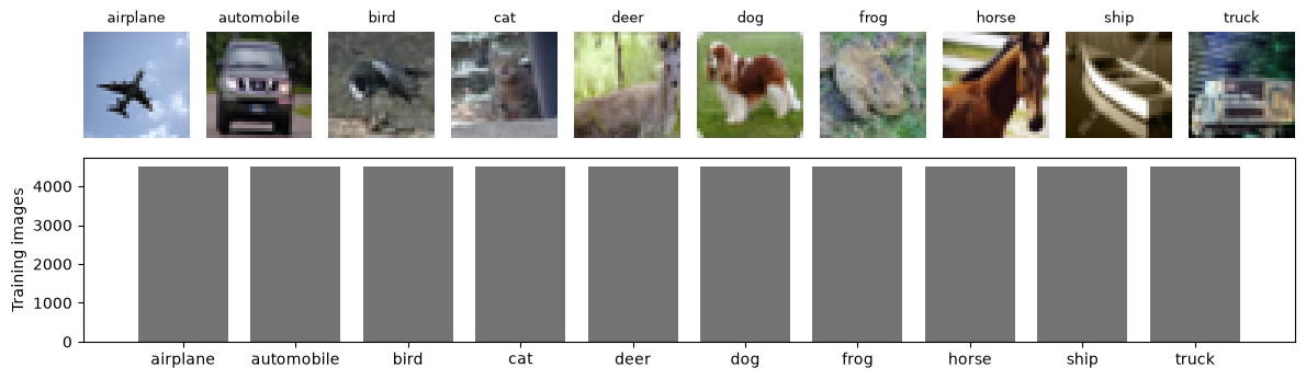
One example per class and the number of training images in each. The classes are balanced, so accuracy is a fair summary of performance.
def as_image(sample):
    # Convert one stored sample to (height, width[, channel]) for plotting.
    if sample.ndim == 1:
        sample = sample.reshape(28, 28)
    if sample.ndim == 3 and sample.shape[0] in (1, 3):
        sample = np.transpose(sample, (1, 2, 0))
    return sample.squeeze()


fig = plt.figure(figsize=(12, 3.6))
grid = fig.add_gridspec(2, 10, height_ratios=[1, 1.2])
for label in range(10):
    axis = fig.add_subplot(grid[0, label])
    image = as_image(x_train[np.flatnonzero(y_train == label)[0]])
    axis.imshow(image, cmap="gray" if image.ndim == 2 else None)
    axis.set_title(CLASS_NAMES[label], fontsize=9)
    axis.axis("off")
counts_axis = fig.add_subplot(grid[1, :])
counts_axis.bar(CLASS_NAMES, np.bincount(y_train, minlength=10), color="0.45")
counts_axis.set(ylabel="Training images")
plt.tight_layout()
plt.show()
Training loop#
Each epoch passes once over the training images in mini-batches. For each
batch, run_epoch computes the cross-entropy loss (the negative
log-probability given to the correct class), backpropagates its gradient, and
lets the Adam optimizer update the weights. After each epoch fit scores the
validation set, and at the end it restores the weights from the epoch with
the best validation accuracy.
loss_function = nn.CrossEntropyLoss()


def make_loader(images, labels, shuffle=False):
    dataset = TensorDataset(torch.from_numpy(images), torch.from_numpy(labels).long())
    generator = torch.Generator().manual_seed(SEED) if shuffle else None
    return DataLoader(dataset, batch_size=BATCH_SIZE, shuffle=shuffle, generator=generator)


def run_epoch(model, loader, optimizer=None):
    # One pass over `loader`; the weights are updated only if an optimizer is given.
    training = optimizer is not None
    model.train(training)
    total_loss, correct = 0.0, 0
    with torch.set_grad_enabled(training):
        for images, labels in loader:
            images, labels = images.to(DEVICE), labels.to(DEVICE)
            logits = model(images)
            loss = loss_function(logits, labels)
            if training:
                optimizer.zero_grad()
                loss.backward()
                optimizer.step()
            total_loss += loss.item() * len(labels)
            correct += (logits.argmax(dim=1) == labels).sum().item()
    return total_loss / len(loader.dataset), correct / len(loader.dataset)


def fit(model, epochs, learning_rate=1e-3, train=None, validation=None, verbose=True):
    # Train with Adam and restore the epoch with the best validation accuracy.
    train_loader = make_loader(*(train or (x_train, y_train)), shuffle=True)
    validation_loader = make_loader(*(validation or (x_validation, y_validation)))
    model.to(DEVICE)
    optimizer = torch.optim.Adam(model.parameters(), lr=learning_rate)
    history = {"loss": [], "accuracy": [], "val_loss": [], "val_accuracy": []}
    best_state, best_accuracy = None, -1.0
    for epoch in range(epochs):
        scores = (*run_epoch(model, train_loader, optimizer), *run_epoch(model, validation_loader))
        for key, value in zip(history, scores):
            history[key].append(value)
        if verbose:
            print(
                f"epoch {epoch + 1:2d}: loss={scores[0]:.4f}  accuracy={scores[1]:.4f}  "
                f"val_loss={scores[2]:.4f}  val_accuracy={scores[3]:.4f}"
            )
        if scores[3] > best_accuracy:
            best_accuracy = scores[3]
            best_state = {key: value.detach().clone() for key, value in model.state_dict().items()}
    model.load_state_dict(best_state)
    if verbose:
        best_epoch = int(np.argmax(history["val_accuracy"])) + 1
        print(f"restored epoch {best_epoch} (validation accuracy {best_accuracy:.4f})")
    return history


def predict_classes(model, images):
    model.eval()
    with torch.no_grad():
        return np.concatenate(
            [model(batch.to(DEVICE)).argmax(dim=1).cpu().numpy()
             for (batch, _) in make_loader(images, np.zeros(len(images), dtype=np.int64))]
        )


def plot_history(history, title=None):
    epochs = np.arange(1, len(history["loss"]) + 1)
    best = epochs[int(np.argmax(history["val_accuracy"]))]
    fig, axes = plt.subplots(1, 2, figsize=(10, 3.4))
    for axis, key, label in zip(axes, ("loss", "accuracy"), ("Cross-entropy loss", "Accuracy")):
        axis.plot(epochs, history[key], marker="o", label="training")
        axis.plot(epochs, history[f"val_{key}"], marker="o", label="validation")
        axis.axvline(best, color="0.6", linestyle=":", label="restored epoch")
        axis.set(title=label, xlabel="Epoch")
        axis.grid(alpha=0.25)
    axes[0].legend()
    if title:
        fig.suptitle(title)
    plt.tight_layout()
    plt.show()
Small network, 5 epochs#
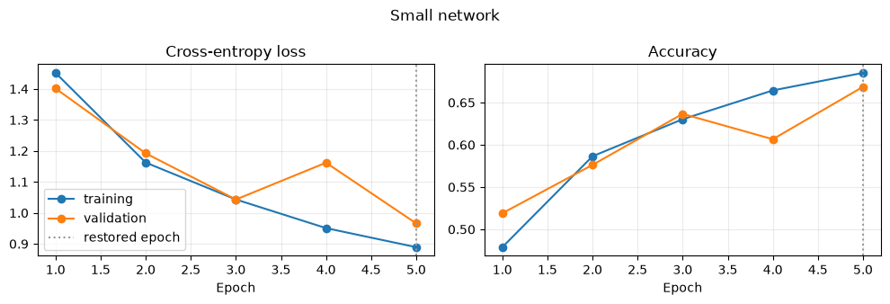
Two convolution layers, the second with stride 2 to halve the resolution, each followed by batch normalization and a leaky ReLU. Batch normalization rescales each layer’s outputs with batch statistics, which stabilizes and speeds up training. One dense layer of 100 units and dropout precede the output.
class SmallNetwork(nn.Module):
    def __init__(self):
        super().__init__()
        self.features = nn.Sequential(
            nn.Conv2d(3, 16, 3), nn.BatchNorm2d(16), nn.LeakyReLU(0.1),
            nn.Conv2d(16, 32, 3, stride=2), nn.BatchNorm2d(32), nn.LeakyReLU(0.1),
        )
        self.classifier = nn.Sequential(
            nn.Flatten(), nn.Linear(32 * 14 * 14, 100), nn.BatchNorm1d(100),
            nn.LeakyReLU(0.1), nn.Dropout(0.5), nn.Linear(100, 10),
        )

    def forward(self, values):
        return self.classifier(self.features(values))


model = SmallNetwork()
print(f"trainable parameters: {sum(p.numel() for p in model.parameters()):,}")
trainable parameters: 633,694
history = fit(model, EPOCHS)
plot_history(history, 'Small network')
small_model, small_history = model, history
small_validation = max(history['val_accuracy'])
epoch 1: loss=1.4518 accuracy=0.4788 val_loss=1.4014 val_accuracy=0.5190
epoch 2: loss=1.1624 accuracy=0.5864 val_loss=1.1922 val_accuracy=0.5762
epoch 3: loss=1.0432 accuracy=0.6303 val_loss=1.0430 val_accuracy=0.6366
epoch 4: loss=0.9508 accuracy=0.6644 val_loss=1.1619 val_accuracy=0.6066
epoch  5: loss=0.8893  accuracy=0.6851  val_loss=0.9661  val_accuracy=0.6686
restored epoch 5 (validation accuracy 0.6686)
Deeper network, 25 epochs#
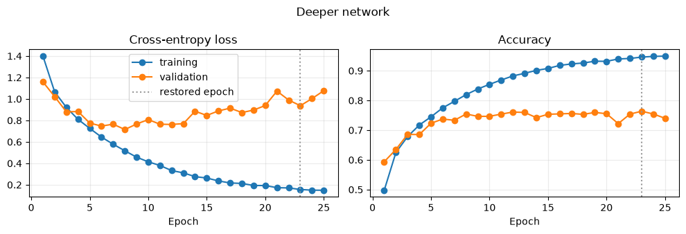
Three convolution stages and dense layers of 600 and 150 units, with dropout after the convolutions and between the dense layers. The extra capacity lets the network learn richer features, but also makes it easier to memorize the training images; the gap between training and validation accuracy shows when that begins.
EPOCHS = 25 # Reduce to 1 or 2 for a quicker run.
class DeeperNetwork(nn.Module):
    def __init__(self):
        super().__init__()
        self.features = nn.Sequential(
            nn.Conv2d(3, 32, 3), nn.BatchNorm2d(32), nn.LeakyReLU(0.1),
            nn.Conv2d(32, 64, 3, stride=2), nn.BatchNorm2d(64), nn.LeakyReLU(0.1),
            nn.Conv2d(64, 128, 3, stride=2), nn.BatchNorm2d(128),
            nn.LeakyReLU(0.1), nn.Dropout(0.2),
        )
        self.classifier = nn.Sequential(
            nn.Flatten(), nn.Linear(128 * 6 * 6, 600), nn.BatchNorm1d(600),
            nn.LeakyReLU(0.1), nn.Dropout(0.25), nn.Linear(600, 150),
            nn.BatchNorm1d(150), nn.LeakyReLU(0.1), nn.Dropout(0.5),
            nn.Linear(150, 10),
        )

    def forward(self, values):
        return self.classifier(self.features(values))


model = DeeperNetwork()
print(f"trainable parameters: {sum(p.numel() for p in model.parameters()):,}")
trainable parameters: 2,952,256
history = fit(model, EPOCHS)
plot_history(history, 'Deeper network')
deeper_model, deeper_history = model, history
deeper_validation = max(history['val_accuracy'])
epoch 1: loss=1.3993 accuracy=0.4977 val_loss=1.1589 val_accuracy=0.5936
epoch 2: loss=1.0661 accuracy=0.6249 val_loss=1.0218 val_accuracy=0.6350
epoch 3: loss=0.9213 accuracy=0.6784 val_loss=0.8800 val_accuracy=0.6858
epoch 4: loss=0.8094 accuracy=0.7173 val_loss=0.8827 val_accuracy=0.6852
epoch 5: loss=0.7258 accuracy=0.7449 val_loss=0.7750 val_accuracy=0.7232
epoch 6: loss=0.6448 accuracy=0.7751 val_loss=0.7473 val_accuracy=0.7374
epoch 7: loss=0.5780 accuracy=0.7971 val_loss=0.7648 val_accuracy=0.7332
epoch 8: loss=0.5169 accuracy=0.8196 val_loss=0.7150 val_accuracy=0.7544
epoch 9: loss=0.4575 accuracy=0.8386 val_loss=0.7661 val_accuracy=0.7464
epoch 10: loss=0.4141 accuracy=0.8543 val_loss=0.8076 val_accuracy=0.7466
epoch 11: loss=0.3801 accuracy=0.8689 val_loss=0.7644 val_accuracy=0.7540
epoch 12: loss=0.3323 accuracy=0.8825 val_loss=0.7625 val_accuracy=0.7610
epoch 13: loss=0.3114 accuracy=0.8914 val_loss=0.7699 val_accuracy=0.7596
epoch 14: loss=0.2758 accuracy=0.9012 val_loss=0.8857 val_accuracy=0.7422
epoch 15: loss=0.2631 accuracy=0.9078 val_loss=0.8464 val_accuracy=0.7534
epoch 16: loss=0.2359 accuracy=0.9181 val_loss=0.8885 val_accuracy=0.7548
epoch 17: loss=0.2169 accuracy=0.9229 val_loss=0.9143 val_accuracy=0.7562
epoch 18: loss=0.2128 accuracy=0.9261 val_loss=0.8732 val_accuracy=0.7532
epoch 19: loss=0.1935 accuracy=0.9320 val_loss=0.8963 val_accuracy=0.7596
epoch 20: loss=0.1927 accuracy=0.9318 val_loss=0.9386 val_accuracy=0.7554
epoch 21: loss=0.1732 accuracy=0.9396 val_loss=1.0731 val_accuracy=0.7220
epoch 22: loss=0.1707 accuracy=0.9414 val_loss=0.9897 val_accuracy=0.7540
epoch 23: loss=0.1562 accuracy=0.9459 val_loss=0.9369 val_accuracy=0.7638
epoch 24: loss=0.1499 accuracy=0.9483 val_loss=1.0038 val_accuracy=0.7544
epoch 25: loss=0.1491  accuracy=0.9493  val_loss=1.0767  val_accuracy=0.7400
restored epoch 23 (validation accuracy 0.7638)
Choose on validation accuracy#
The choice between the two networks uses the validation set only, so the test score of the chosen network remains an unbiased estimate.
if deeper_validation > small_validation:
    selected_name, model = "deeper network", deeper_model
else:
    selected_name, model = "small network", small_model
fig, ax = plt.subplots(figsize=(7, 3.4))
ax.plot(np.arange(1, len(small_history["val_accuracy"]) + 1), small_history["val_accuracy"], marker="o", label="small (5 epochs)")
ax.plot(np.arange(1, len(deeper_history["val_accuracy"]) + 1), deeper_history["val_accuracy"], marker="o", label="deeper (25 epochs)")
ax.set(title="Validation accuracy", xlabel="Epoch", ylabel="Accuracy")
ax.legend()
ax.grid(alpha=0.25)
plt.show()
print(
    f"best validation accuracy: small {small_validation:.4f}, deeper {deeper_validation:.4f}; "
    f"selected: {selected_name}"
)
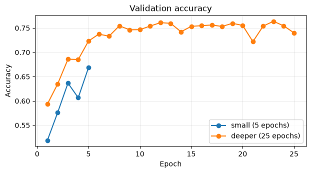
best validation accuracy: small 0.6686, deeper 0.7638; selected: deeper network
Evaluate the chosen network on the test set#
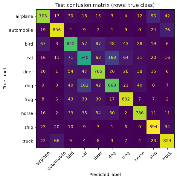
The confusion matrix shows which classes are mistaken for which.
test_predictions = predict_classes(model, x_test)
test_accuracy = accuracy_score(y_test, test_predictions)
cm = confusion_matrix(y_test, test_predictions, labels=np.arange(10))
print(f"test accuracy: {test_accuracy:.4f}")
print(
    classification_report(
        y_test, test_predictions, labels=np.arange(10),
        target_names=CLASS_NAMES, digits=3, zero_division=0,
    )
)

fig, ax = plt.subplots(figsize=(7, 6))
ConfusionMatrixDisplay(cm, display_labels=CLASS_NAMES).plot(
    ax=ax, colorbar=False, values_format="d", xticks_rotation=45
)
ax.set_title("Test confusion matrix (rows: true class)")
plt.show()

mistakes = np.flatnonzero(test_predictions != y_test)[:12]
fig, axes = plt.subplots(2, 6, figsize=(12, 4.6))
for axis in axes.flat:
    axis.axis("off")
for axis, index in zip(axes.flat, mistakes):
    image = as_image(x_test[index])
    axis.imshow(image, cmap="gray" if image.ndim == 2 else None)
    axis.set_title(f"{CLASS_NAMES[y_test[index]]} as {CLASS_NAMES[test_predictions[index]]}", fontsize=9)
fig.suptitle("First twelve test mistakes (true as predicted)")
plt.tight_layout()
plt.show()
test accuracy: 0.7600
              precision    recall  f1-score   support

    airplane      0.792     0.763     0.777      1000
  automobile      0.869     0.856     0.862      1000
        bird      0.686     0.642     0.663      1000
         cat      0.587     0.540     0.562      1000
        deer      0.710     0.765     0.736      1000
         dog      0.678     0.668     0.673      1000
        frog      0.819     0.832     0.825      1000
       horse      0.831     0.786     0.808      1000
        ship      0.800     0.894     0.845      1000
       truck      0.810     0.854     0.832      1000

    accuracy                          0.760     10000
   macro avg      0.758     0.760     0.758     10000
weighted avg      0.758     0.760     0.758     10000
What the results show#
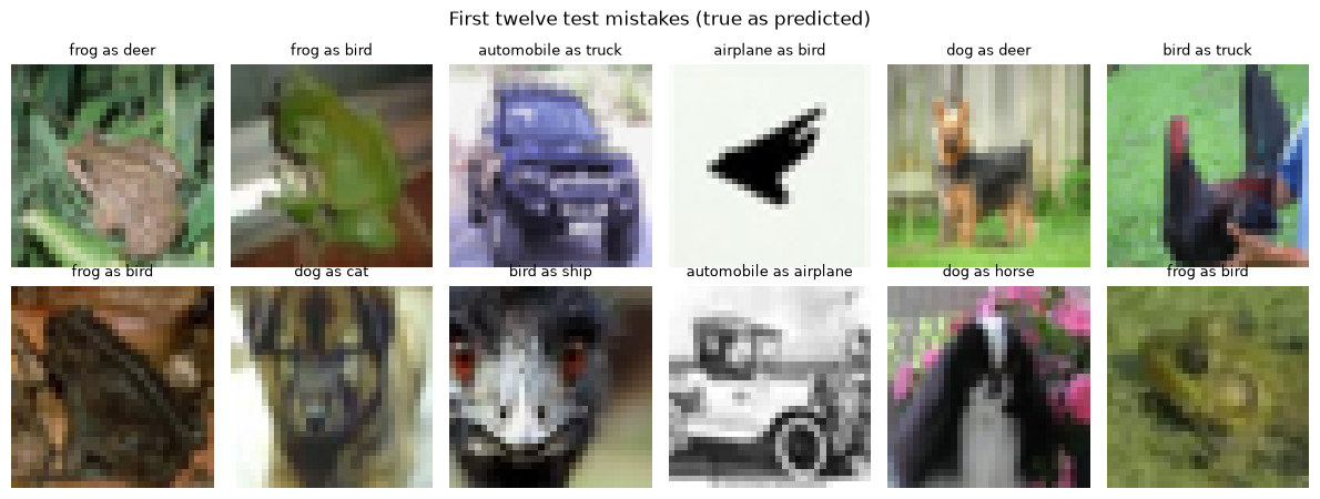
In both saved runs, validation selects the deeper network. Training accuracy continues to improve while validation accuracy levels off, and the best checkpoint occurs before the final epoch. Cats have the lowest test recall. The models also receive different training budgets (5 versus 25 epochs), so the comparison does not isolate network depth. Try training-image flips and crops as a next step, keeping validation and test images unchanged.
Try it yourself#
Change one choice at a time and keep the data split and evaluation unchanged:
add random horizontal flips to the training images of the deeper network and compare the learning curves.
change the dropout rates of the deeper network and see where overfitting starts.
train the small network for 25 epochs to separate the effect of capacity from that of training time.