
Coronal-Loop Reconstruction: PyTorch#
EUV imagers see coronal loops only in projection. This notebook asks whether a network can recover the height profile \(z(s)\) of a loop from its projected shape and three scalar descriptors, following Chifu and Gafeira (2021). The data are 5,000 loops, each sampled at 1,500 points.
The answer depends on which loops the model is tested on. Neighbouring loops in the archive are nearly identical, and the archive is ordered by position, so we compare three splits: random loops, groups of 50 consecutive loops, and one contiguous spatial block.
Imports#
A fixed seed makes repeated runs comparable.
Load the loops#
The arrays are downloaded once and checked against their SHA-256 checksums.
verified dataset: coronal-loops
  X2D.npy (checksum verified)
  Y2D.npy (checksum verified)
  LNGTH_L2D.npy (checksum verified)
  DST2D_FP.npy (checksum verified)
  angle_top.npy (checksum verified)
  Z3D.npy (checksum verified)
Describe each loop by its shape#
A loop’s height depends on its geometry, not on where it sits on the disk. We therefore rotate and translate each projected loop into a frame fixed by its footpoints and add the archived projected length, footpoint separation, and apex angle as extra channels. The target is the height at each of the 1,500 points.
x_coordinates = np.load(dataset_files["X2D.npy"], mmap_mode="r")
y_coordinates = np.load(dataset_files["Y2D.npy"], mmap_mode="r")
z_coordinates = np.load(dataset_files["Z3D.npy"], mmap_mode="r")
length = np.load(dataset_files["LNGTH_L2D.npy"]).astype(np.float32)
footpoint_distance = np.load(dataset_files["DST2D_FP.npy"]).astype(np.float32)
top_angle = np.load(dataset_files["angle_top.npy"]).astype(np.float32)

# The arrays store one loop per column; transpose to (loop, point).
point_slice = slice(None)
x_projected = np.asarray(x_coordinates[point_slice], dtype=np.float32).T
y_projected = np.asarray(y_coordinates[point_slice], dtype=np.float32).T
heights = np.asarray(z_coordinates[point_slice], dtype=np.float32).T
loop_count, point_count = heights.shape

# Express each projected loop in its own footpoint frame: `along` runs parallel
# to the line joining the two footpoints and `across` is perpendicular to it.
# The network then sees the shape of a loop, not its position on the disk.
baseline_x = x_projected[:, -1:] - x_projected[:, :1]
baseline_y = y_projected[:, -1:] - y_projected[:, :1]
baseline_length = np.hypot(baseline_x, baseline_y)
unit_x, unit_y = baseline_x / baseline_length, baseline_y / baseline_length
relative_x = x_projected - x_projected[:, :1]
relative_y = y_projected - y_projected[:, :1]
along = relative_x * unit_x + relative_y * unit_y
across = relative_y * unit_x - relative_x * unit_y
descriptors = np.stack([length, footpoint_distance, top_angle], axis=1)
features = np.concatenate(
    [
        along[..., None],
        across[..., None],
        np.repeat(descriptors[:, None, :], point_count, axis=1),
    ],
    axis=2,
).astype(np.float32)
print(
    f"loops={loop_count:,}, points per loop={point_count}, "
    f"input channels={features.shape[2]} (along, across, length, "
    "footpoint distance, apex angle)"
)
loops=5,000, points per loop=1500, input channels=5 (along, across, length, footpoint distance, apex angle)
Three ways to split the loops#
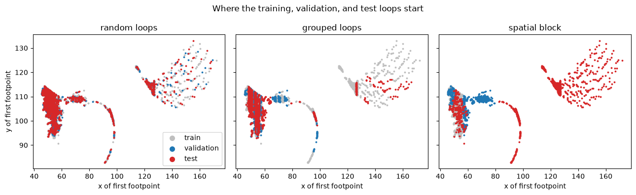
Random loops assigns individual loops at random. Because a loop’s neighbours are near-copies of it, the test set contains close relatives of training loops, and the score is optimistic.
Grouped loops assigns blocks of 50 consecutive loops at random. Loops within each block stay together, but similar loops may cross its boundaries. This is a split-sensitivity check, not a guarantee of independent regions.
Spatial block keeps the archive order: the first 60% train, the next 15% validate, and the last 25% test. The test loops come from a region the model has never seen, so this measures extrapolation.
GROUP_SIZE = 50  # Consecutive loops kept together in the grouped split.
rng = np.random.default_rng(SEED)
n_train, n_validation = int(0.60 * loop_count), int(0.15 * loop_count)


def by_fraction(order):
    return (
        np.sort(order[:n_train]),
        np.sort(order[n_train : n_train + n_validation]),
        np.sort(order[n_train + n_validation :]),
    )


group_order = rng.permutation(loop_count // GROUP_SIZE)
grouped_order = np.concatenate(
    [np.arange(group * GROUP_SIZE, (group + 1) * GROUP_SIZE) for group in group_order]
)
splits = {
    "random loops": by_fraction(rng.permutation(loop_count)),
    "grouped loops": by_fraction(grouped_order),
    "spatial block": by_fraction(np.arange(loop_count)),
}
for name, (train, validation, test) in splits.items():
    assert not set(train) & set(test) and not set(validation) & set(test)
    print(f"{name:14s} train={len(train):,}  validation={len(validation):,}  test={len(test):,}")

neighbour_gap = np.abs(heights[1:] - heights[:-1]).mean(axis=1)
print(
    "median mean-absolute height difference between neighbouring loops: "
    f"{np.median(neighbour_gap):.3f} (typical apex height {np.median(heights.max(axis=1)):.1f})"
)

fig, axes = plt.subplots(1, 3, figsize=(13, 4), sharex=True, sharey=True)
roles = (("train", "0.75"), ("validation", "tab:blue"), ("test", "tab:red"))
for axis, (name, members) in zip(axes, splits.items()):
    for (role, color), indices in zip(roles, members):
        axis.scatter(
            x_projected[indices, 0], y_projected[indices, 0],
            s=3, color=color, label=role, rasterized=True,
        )
    axis.set(title=name, xlabel="x of first footpoint")
axes[0].set_ylabel("y of first footpoint")
axes[0].legend(markerscale=4, loc="lower right")
fig.suptitle("Where the training, validation, and test loops start")
plt.tight_layout()
plt.show()
random loops   train=3,000  validation=750  test=1,250
grouped loops  train=3,000  validation=750  test=1,250
spatial block  train=3,000  validation=750  test=1,250
median mean-absolute height difference between neighbouring loops: 0.197 (typical apex height 12.4)
Normalize within each split#
Inputs are standardized per channel and heights per point, using the training loops of the split in question.
def prepare_split(split):
    train, validation, test = split
    # Normalization statistics come from the training loops of this split only.
    feature_mean = features[train].mean(axis=(0, 1), keepdims=True)
    feature_std = features[train].std(axis=(0, 1), keepdims=True)
    feature_std[feature_std < 1e-6] = 1.0
    target_mean = heights[train].mean(axis=0, keepdims=True)
    target_std = heights[train].std(axis=0, keepdims=True)
    target_std[target_std < 1e-6] = 1.0

    def scale_x(indices):
        return ((features[indices] - feature_mean) / feature_std).astype(np.float32)

    def scale_y(indices):
        return ((heights[indices] - target_mean) / target_std).astype(np.float32)

    return {
        "x_train": scale_x(train), "y_train": scale_y(train),
        "x_validation": scale_x(validation), "y_validation": scale_y(validation),
        "x_test": scale_x(test), "y_test": heights[test],
        "target_mean": target_mean, "target_std": target_std,
    }
Define the PyTorch regressor#
Three convolution and pooling stages summarize the loop; a dense layer maps that summary to all 1,500 heights. Training stops when the validation loss has not improved for three epochs, and the best state is restored.
import torch
from torch import nn
from torch.utils.data import DataLoader, TensorDataset

EPOCHS = 10  # Reduce to 3 or 5 for a quicker run.
PATIENCE = 3
os.environ.setdefault("CUBLAS_WORKSPACE_CONFIG", ":4096:8")  # Deterministic cuBLAS on GPUs.
torch.use_deterministic_algorithms(True, warn_only=True)
DEVICE = torch.device(
    "cuda" if torch.cuda.is_available()
    else "mps" if torch.backends.mps.is_available()
    else "cpu"
)


# Define the neural network used to reconstruct the loop height profile:
# 1-D convolutions read the ordered points, a dense head returns all heights.
class LoopRegressor(nn.Module):
    def __init__(self, input_channels, output_points):
        super().__init__()
        self.features = nn.Sequential(
            nn.Conv1d(input_channels, 32, 25, padding=12), nn.ReLU(), nn.MaxPool1d(4),
            nn.Conv1d(32, 64, 15, padding=7), nn.ReLU(), nn.MaxPool1d(4),
            nn.Conv1d(64, 64, 7, padding=3), nn.ReLU(), nn.AdaptiveAvgPool1d(1),
        )
        self.regressor = nn.Sequential(
            nn.Flatten(), nn.Linear(64, 256), nn.ReLU(), nn.Linear(256, output_points)
        )

    def forward(self, inputs):
        return self.regressor(self.features(inputs.transpose(1, 2)))


def train_regressor(data):
    torch.manual_seed(SEED)
    model = LoopRegressor(features.shape[2], point_count).to(DEVICE)
    optimizer = torch.optim.Adam(model.parameters())
    loss_function = nn.MSELoss()
    loader = DataLoader(
        TensorDataset(torch.from_numpy(data["x_train"]), torch.from_numpy(data["y_train"])),
        batch_size=32,
        shuffle=True,
        generator=torch.Generator().manual_seed(SEED),
    )
    x_validation = torch.from_numpy(data["x_validation"]).to(DEVICE)
    y_validation = torch.from_numpy(data["y_validation"]).to(DEVICE)
    losses = {"loss": [], "val_loss": []}
    best_state, best_loss, stale_epochs = None, float("inf"), 0
    for epoch in range(EPOCHS):
        model.train()
        total = 0.0
        for batch_x, batch_y in loader:
            optimizer.zero_grad()
            loss = loss_function(model(batch_x.to(DEVICE)), batch_y.to(DEVICE))
            loss.backward()
            optimizer.step()
            total += loss.item() * len(batch_x)
        model.eval()
        with torch.no_grad():
            validation_loss = loss_function(model(x_validation), y_validation).item()
        losses["loss"].append(total / len(loader.dataset))
        losses["val_loss"].append(validation_loss)
        if validation_loss < best_loss:
            best_loss, stale_epochs = validation_loss, 0
            best_state = {key: value.detach().clone() for key, value in model.state_dict().items()}
        else:
            stale_epochs += 1
            if stale_epochs >= PATIENCE:
                break
    model.load_state_dict(best_state)
    model.eval()

    def predict(x):
        with torch.no_grad():
            return model(torch.from_numpy(x).to(DEVICE)).cpu().numpy()

    return predict, losses
Train and evaluate under each split#
The reference prediction is the mean training height at each point along the loop. A skill above zero means the model beats that profile; R² is computed over all points of all test loops.
def rmse(y_true, y_prediction):
    return float(mean_squared_error(y_true.ravel(), y_prediction.ravel()) ** 0.5)


runs, rows = {}, []
for name, split in splits.items():
    data = prepare_split(split)
    predict, losses = train_regressor(data)
    predictions = predict(data["x_test"]) * data["target_std"] + data["target_mean"]
    # Reference: predict the mean training height at every point along the loop.
    baseline = np.repeat(data["target_mean"], len(split[2]), axis=0)
    model_rmse, baseline_rmse = rmse(data["y_test"], predictions), rmse(data["y_test"], baseline)
    runs[name] = {"predictions": predictions, "losses": losses, "test": split[2]}
    rows.append(
        {
            "split": name,
            "model RMSE": model_rmse,
            "mean-profile RMSE": baseline_rmse,
            "model R²": float(r2_score(data["y_test"].ravel(), predictions.ravel())),
            "skill vs mean profile": 1.0 - model_rmse**2 / baseline_rmse**2,
            "epochs": len(losses["loss"]),
        }
    )
    print(f"{name}: model RMSE {model_rmse:.2f}, mean-profile RMSE {baseline_rmse:.2f}")

summary = pd.DataFrame(rows).set_index("split")
display(summary.round(3))
random loops: model RMSE 0.65, mean-profile RMSE 2.94
grouped loops: model RMSE 1.28, mean-profile RMSE 2.24
spatial block: model RMSE 4.11, mean-profile RMSE 1.99
| model RMSE | mean-profile RMSE | model R² | skill vs mean profile | epochs | |
|---|---|---|---|---|---|
| split | |||||
| random loops | 0.650 | 2.939 | 0.983 | 0.951 | 10 |
| grouped loops | 1.282 | 2.243 | 0.917 | 0.673 | 7 |
| spatial block | 4.106 | 1.991 | 0.041 | -3.251 | 4 |
Learning curves and example reconstructions#
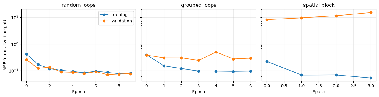
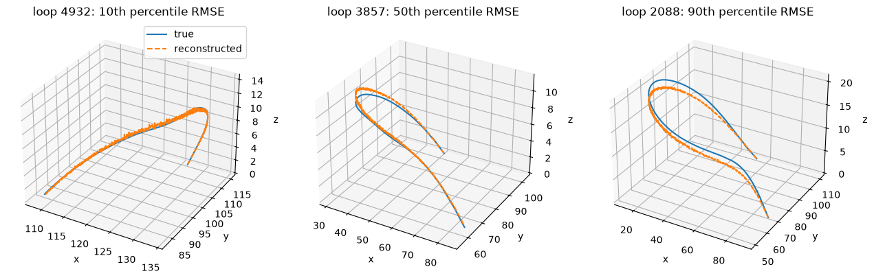
The upper panels compare training and validation loss for each split. The lower panels show grouped-split test loops at the 10th, 50th, and 90th percentiles of loop RMSE.
fig, axes = plt.subplots(1, 3, figsize=(13, 3.4), sharey=True)
for axis, (name, run) in zip(axes, runs.items()):
    axis.plot(run["losses"]["loss"], marker="o", label="training")
    axis.plot(run["losses"]["val_loss"], marker="o", label="validation")
    axis.set(title=name, xlabel="Epoch", yscale="log")
    axis.grid(alpha=0.25)
axes[0].set_ylabel("MSE (normalized height)")
axes[0].legend()
plt.tight_layout()
plt.show()

grouped = runs["grouped loops"]
grouped_heights = heights[grouped["test"]]
loop_rmse = np.sqrt(np.mean((grouped_heights - grouped["predictions"]) ** 2, axis=1))
examples = np.argsort(loop_rmse)[[len(loop_rmse) // 10, len(loop_rmse) // 2, -len(loop_rmse) // 10]]

fig = plt.figure(figsize=(13, 4))
for panel, (index, label) in enumerate(zip(examples, ("10th", "50th", "90th")), start=1):
    loop = grouped["test"][index]
    axis = fig.add_subplot(1, 3, panel, projection="3d")
    axis.plot(x_projected[loop], y_projected[loop], heights[loop], label="true")
    axis.plot(
        x_projected[loop], y_projected[loop], grouped["predictions"][index],
        linestyle="--", label="reconstructed",
    )
    axis.set(title=f"loop {loop}: {label} percentile RMSE", xlabel="x", ylabel="y", zlabel="z")
fig.axes[0].legend()
plt.tight_layout()
plt.show()
What the results show#
With random loops, the network appears almost perfect. That number is inflated: most test loops have a neighbour in the training set whose heights differ by about 0.2, or 2% of a typical apex height. Grouping 50 consecutive loops tests sensitivity to the split, but similar loops can still cross group boundaries; it does not establish independent test regions.
The spatial block is a different question. Its test loops are shorter and relatively taller than typical training loops, and the model does not beat the mean profile there. These runs do not establish which model or data changes would improve extrapolation.