
CIFAR-10 Transfer Learning: PyTorch#
Transfer learning reuses a network trained on one large dataset as a feature extractor for a new task. Here the convolutional part of VGG16, trained on 1.3 million ImageNet photographs, is frozen, and only a small classifier on top of it is trained. The benefit should be largest when labelled examples are scarce, which is the usual situation for rare heliophysical events. We therefore train on 1,000, 5,000, and 45,000 CIFAR-10 images and compare with the small CNN of the CIFAR-10 progression trained from scratch on the same images.
The pretrained weights (about 500 MB) are downloaded on first use. Feature extraction takes several minutes on a CPU.
Setup#
The libraries used below.
PyTorch 2.13.0
Load CIFAR-10 and split it#
The 50,000 official training images are split, with a fixed seed and stratified by class, into 45,000 for training and 5,000 for validation. The 10,000 official test images are used once, at the end.
SEED = 42
EPOCHS = 10  # Reduce to 1 or 2 for a quicker run.
BATCH_SIZE = 256
CLASS_NAMES = ['airplane', 'automobile', 'bird', 'cat', 'deer', 'dog', 'frog', 'horse', 'ship', 'truck']

random.seed(SEED)
np.random.seed(SEED)
torch.manual_seed(SEED)
os.environ.setdefault("CUBLAS_WORKSPACE_CONFIG", ":4096:8")  # Deterministic cuBLAS on GPUs.
torch.use_deterministic_algorithms(True, warn_only=True)
DEVICE = torch.device(
    "cuda" if torch.cuda.is_available()
    else "mps" if torch.backends.mps.is_available()
    else "cpu"
)


data_root = Path(
    os.getenv("HELIO_DATA_DIR", Path.home() / ".cache" / "helio-data-methods")
)
development_dataset = datasets.CIFAR10(data_root, train=True, download=True)
test_dataset = datasets.CIFAR10(data_root, train=False, download=True)
x_development = development_dataset.data
y_development = np.asarray(development_dataset.targets)
x_test = test_dataset.data
y_test = np.asarray(test_dataset.targets)

all_indices = np.arange(len(y_development))
train_indices, validation_indices = train_test_split(
    all_indices,
    test_size=5000,
    random_state=SEED,
    stratify=y_development,
)
split_signature = hashlib.sha256(
    validation_indices.astype("<i8").tobytes()
).hexdigest()[:16]

# Scale pixel values from 0-255 to 0-1.
x_train = x_development[train_indices].astype("float32") / 255.0
y_train = y_development[train_indices].astype(np.int64)
x_validation = x_development[validation_indices].astype("float32") / 255.0
y_validation = y_development[validation_indices].astype(np.int64)
x_test = x_test.astype("float32") / 255.0
y_test = y_test.astype(np.int64)
# PyTorch expects (sample, channel, height, width).
x_train = np.transpose(x_train, (0, 3, 1, 2))
x_validation = np.transpose(x_validation, (0, 3, 1, 2))
x_test = np.transpose(x_test, (0, 3, 1, 2))

assert set(train_indices).isdisjoint(validation_indices)
print(
    f"train={len(y_train):,}, validation={len(y_validation):,}, "
    f"test={len(y_test):,}, image shape={x_train.shape[1:]}"
)
train=45,000, validation=5,000, test=10,000, image shape=(3, 32, 32)
Look at the data#
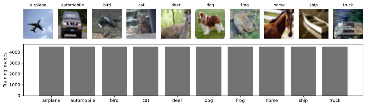
One example per class and the number of training images in each. The classes are balanced, so accuracy is a fair summary of performance.
def as_image(sample):
    # Convert one stored sample to (height, width[, channel]) for plotting.
    if sample.ndim == 1:
        sample = sample.reshape(28, 28)
    if sample.ndim == 3 and sample.shape[0] in (1, 3):
        sample = np.transpose(sample, (1, 2, 0))
    return sample.squeeze()


fig = plt.figure(figsize=(12, 3.6))
grid = fig.add_gridspec(2, 10, height_ratios=[1, 1.2])
for label in range(10):
    axis = fig.add_subplot(grid[0, label])
    image = as_image(x_train[np.flatnonzero(y_train == label)[0]])
    axis.imshow(image, cmap="gray" if image.ndim == 2 else None)
    axis.set_title(CLASS_NAMES[label], fontsize=9)
    axis.axis("off")
counts_axis = fig.add_subplot(grid[1, :])
counts_axis.bar(CLASS_NAMES, np.bincount(y_train, minlength=10), color="0.45")
counts_axis.set(ylabel="Training images")
plt.tight_layout()
plt.show()
Training loop#
Each epoch passes once over the training images in mini-batches. For each
batch, run_epoch computes the cross-entropy loss (the negative
log-probability given to the correct class), backpropagates its gradient, and
lets the Adam optimizer update the weights. After each epoch fit scores the
validation set, and at the end it restores the weights from the epoch with
the best validation accuracy.
loss_function = nn.CrossEntropyLoss()


def make_loader(images, labels, shuffle=False):
    dataset = TensorDataset(torch.from_numpy(images), torch.from_numpy(labels).long())
    generator = torch.Generator().manual_seed(SEED) if shuffle else None
    return DataLoader(dataset, batch_size=BATCH_SIZE, shuffle=shuffle, generator=generator)


def run_epoch(model, loader, optimizer=None):
    # One pass over `loader`; the weights are updated only if an optimizer is given.
    training = optimizer is not None
    model.train(training)
    total_loss, correct = 0.0, 0
    with torch.set_grad_enabled(training):
        for images, labels in loader:
            images, labels = images.to(DEVICE), labels.to(DEVICE)
            logits = model(images)
            loss = loss_function(logits, labels)
            if training:
                optimizer.zero_grad()
                loss.backward()
                optimizer.step()
            total_loss += loss.item() * len(labels)
            correct += (logits.argmax(dim=1) == labels).sum().item()
    return total_loss / len(loader.dataset), correct / len(loader.dataset)


def fit(model, epochs, learning_rate=1e-3, train=None, validation=None, verbose=True):
    # Train with Adam and restore the epoch with the best validation accuracy.
    train_loader = make_loader(*(train or (x_train, y_train)), shuffle=True)
    validation_loader = make_loader(*(validation or (x_validation, y_validation)))
    model.to(DEVICE)
    optimizer = torch.optim.Adam(model.parameters(), lr=learning_rate)
    history = {"loss": [], "accuracy": [], "val_loss": [], "val_accuracy": []}
    best_state, best_accuracy = None, -1.0
    for epoch in range(epochs):
        scores = (*run_epoch(model, train_loader, optimizer), *run_epoch(model, validation_loader))
        for key, value in zip(history, scores):
            history[key].append(value)
        if verbose:
            print(
                f"epoch {epoch + 1:2d}: loss={scores[0]:.4f}  accuracy={scores[1]:.4f}  "
                f"val_loss={scores[2]:.4f}  val_accuracy={scores[3]:.4f}"
            )
        if scores[3] > best_accuracy:
            best_accuracy = scores[3]
            best_state = {key: value.detach().clone() for key, value in model.state_dict().items()}
    model.load_state_dict(best_state)
    if verbose:
        best_epoch = int(np.argmax(history["val_accuracy"])) + 1
        print(f"restored epoch {best_epoch} (validation accuracy {best_accuracy:.4f})")
    return history


def predict_classes(model, images):
    model.eval()
    with torch.no_grad():
        return np.concatenate(
            [model(batch.to(DEVICE)).argmax(dim=1).cpu().numpy()
             for (batch, _) in make_loader(images, np.zeros(len(images), dtype=np.int64))]
        )


def plot_history(history, title=None):
    epochs = np.arange(1, len(history["loss"]) + 1)
    best = epochs[int(np.argmax(history["val_accuracy"]))]
    fig, axes = plt.subplots(1, 2, figsize=(10, 3.4))
    for axis, key, label in zip(axes, ("loss", "accuracy"), ("Cross-entropy loss", "Accuracy")):
        axis.plot(epochs, history[key], marker="o", label="training")
        axis.plot(epochs, history[f"val_{key}"], marker="o", label="validation")
        axis.axvline(best, color="0.6", linestyle=":", label="restored epoch")
        axis.set(title=label, xlabel="Epoch")
        axis.grid(alpha=0.25)
    axes[0].legend()
    if title:
        fig.suptitle(title)
    plt.tight_layout()
    plt.show()
Extract frozen VGG16 features#
Each image is enlarged to 64×64 pixels, normalized as VGG16 expects, and passed once through the frozen convolutional layers. Averaging the last feature maps gives a 512-number summary per image. Only the small head defined here is trained.
from torchvision.models import VGG16_Weights, vgg16

IMAGE_SIZE = 64  # VGG16 was trained on 224-pixel images; 32 pixels leaves a 1x1 map.
HEAD_EPOCHS = 30
SUBSET_SIZES = [1_000, 5_000, 45_000]
imagenet_mean = torch.tensor([0.485, 0.456, 0.406]).view(1, 3, 1, 1)
imagenet_std = torch.tensor([0.229, 0.224, 0.225]).view(1, 3, 1, 1)

backbone = vgg16(weights=VGG16_Weights.DEFAULT).features.to(DEVICE).eval()
for parameter in backbone.parameters():
    parameter.requires_grad = False  # Freeze the pretrained filters.


def extract_features(images):
    # Resize, normalize with ImageNet statistics, and average-pool VGG16's last maps.
    outputs = []
    with torch.no_grad():
        for start in range(0, len(images), 256):
            batch = torch.from_numpy(images[start : start + 256])
            batch = nn.functional.interpolate(batch, size=IMAGE_SIZE, mode="bilinear")
            batch = ((batch - imagenet_mean) / imagenet_std).to(DEVICE)
            outputs.append(backbone(batch).mean(dim=(2, 3)).cpu().numpy())
    return np.concatenate(outputs).astype(np.float32)


started = time.perf_counter()
features_train = extract_features(x_train)
features_validation = extract_features(x_validation)
features_test = extract_features(x_test)
print(
    f"feature vectors: {features_train.shape[1]} per image; "
    f"extraction took {time.perf_counter() - started:.0f} s"
)


def make_head():
    # The only trainable part of the transfer model.
    return nn.Sequential(
        nn.Linear(512, 256), nn.ReLU(), nn.Dropout(0.25), nn.Linear(256, 10)
    )
feature vectors: 512 per image; extraction took 21 s
The comparison network#
The same small CNN as in the CIFAR-10 progression, trained from raw pixels for 10 epochs.
class SmallNetwork(nn.Module):
    def __init__(self):
        super().__init__()
        self.features = nn.Sequential(
            nn.Conv2d(3, 16, 3), nn.BatchNorm2d(16), nn.LeakyReLU(0.1),
            nn.Conv2d(16, 32, 3, stride=2), nn.BatchNorm2d(32), nn.LeakyReLU(0.1),
        )
        self.classifier = nn.Sequential(
            nn.Flatten(), nn.Linear(32 * 14 * 14, 100), nn.BatchNorm1d(100),
            nn.LeakyReLU(0.1), nn.Dropout(0.5), nn.Linear(100, 10),
        )

    def forward(self, values):
        return self.classifier(self.features(values))


def make_scratch_network():
    return SmallNetwork()


model = SmallNetwork()
print(f"trainable parameters: {sum(p.numel() for p in model.parameters()):,}")
trainable parameters: 633,694
Train both on growing subsets#
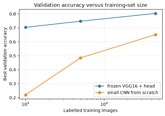
For each subset size, both models see the same training images and are scored on the full validation set. The frozen-feature head receives 30 epochs and the scratch CNN 10; this compares two practical training setups, not the effect of pretraining alone. The test set is not used here.
rows, heads = [], {}
for size in sorted({min(size, len(y_train)) for size in SUBSET_SIZES}):
    subset = np.arange(size)  # The training order is already shuffled.
    head = make_head()
    head_history = fit(
        head, HEAD_EPOCHS,
        train=(features_train[subset], y_train[subset]),
        validation=(features_validation, y_validation),
        verbose=False,
    )
    scratch = make_scratch_network()
    scratch_history = fit(
        scratch, EPOCHS, train=(x_train[subset], y_train[subset]), verbose=False
    )
    heads[size] = head
    rows.append(
        {
            "training images": size,
            "frozen VGG16 + head": max(head_history["val_accuracy"]),
            "small CNN from scratch": max(scratch_history["val_accuracy"]),
        }
    )
    print(f"{size:>6,} images: transfer {rows[-1]['frozen VGG16 + head']:.3f}, "
          f"scratch {rows[-1]['small CNN from scratch']:.3f}")

comparison = pd.DataFrame(rows).set_index("training images")
display(comparison.round(3))
fig, ax = plt.subplots(figsize=(6, 3.8))
for column in comparison:
    ax.plot(comparison.index, comparison[column], marker="o", label=column)
ax.set(
    xscale="log", xlabel="Labelled training images", ylabel="Best validation accuracy",
    title="Validation accuracy versus training-set size",
)
ax.legend()
ax.grid(alpha=0.25)
plt.show()
1,000 images: transfer 0.703, scratch 0.220
5,000 images: transfer 0.747, scratch 0.484
45,000 images: transfer 0.803, scratch 0.652
| frozen VGG16 + head | small CNN from scratch | |
|---|---|---|
| training images | ||
| 1000 | 0.703 | 0.220 |
| 5000 | 0.747 | 0.484 |
| 45000 | 0.803 | 0.652 |
Evaluate the transfer model on the test set#
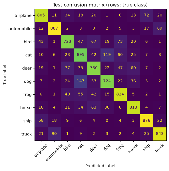
The head trained on all 45,000 images is evaluated once.
model = heads[max(heads)]
test_predictions = predict_classes(model, features_test)
test_accuracy = accuracy_score(y_test, test_predictions)
cm = confusion_matrix(y_test, test_predictions, labels=np.arange(10))
print(f"test accuracy: {test_accuracy:.4f}")
print(
    classification_report(
        y_test, test_predictions, labels=np.arange(10),
        target_names=CLASS_NAMES, digits=3, zero_division=0,
    )
)

fig, ax = plt.subplots(figsize=(7, 6))
ConfusionMatrixDisplay(cm, display_labels=CLASS_NAMES).plot(
    ax=ax, colorbar=False, values_format="d", xticks_rotation=45
)
ax.set_title("Test confusion matrix (rows: true class)")
plt.show()

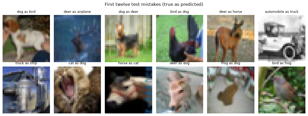
mistakes = np.flatnonzero(test_predictions != y_test)[:12]
fig, axes = plt.subplots(2, 6, figsize=(12, 4.6))
for axis in axes.flat:
    axis.axis("off")
for axis, index in zip(axes.flat, mistakes):
    image = as_image(x_test[index])
    axis.imshow(image, cmap="gray" if image.ndim == 2 else None)
    axis.set_title(f"{CLASS_NAMES[y_test[index]]} as {CLASS_NAMES[test_predictions[index]]}", fontsize=9)
fig.suptitle("First twelve test mistakes (true as predicted)")
plt.tight_layout()
plt.show()
test accuracy: 0.7920
              precision    recall  f1-score   support

    airplane      0.806     0.805     0.805      1000
  automobile      0.869     0.887     0.878      1000
        bird      0.747     0.723     0.735      1000
         cat      0.663     0.695     0.678      1000
        deer      0.728     0.730     0.729      1000
         dog      0.774     0.724     0.748      1000
        frog      0.786     0.824     0.804      1000
       horse      0.828     0.813     0.820      1000
        ship      0.860     0.876     0.868      1000
       truck      0.865     0.843     0.854      1000

    accuracy                          0.792     10000
   macro avg      0.792     0.792     0.792     10000
weighted avg      0.792     0.792     0.792     10000
What the results show#
In the saved runs, the frozen VGG16 features give higher validation accuracy at all three training-set sizes. Their advantage is smaller at 45,000 images than at either smaller subset, although the changes are not monotonic in both implementations. The head and scratch network have different training budgets; this is not a controlled measurement of pretraining alone.
Each library uses its own ImageNet VGG16 weights and matching preprocessing, so the PyTorch and Keras scores need not match.
Try it yourself#
Change one choice at a time and keep the data split and evaluation unchanged:
add a 250-image subset to
SUBSET_SIZESto see how far the frozen features carry.replace the head with a single linear layer, a logistic regression on the VGG16 features.
for a larger extension, replace cached-feature training with an end-to-end image model, unfreeze the last VGG16 block, and try a learning rate of
1e-5.