
SEP Occurrence Forecasting: Keras 3#
The data come from Aminalragia-Giamini et al. (2021), who predicted solar energetic particle (SEP) events from soft X-ray flare measurements. Each sample has 49 standardized predictors and a binary label. The archive has no column names, event identifiers, or timestamps, so two limits apply throughout: predictors cannot be interpreted physically, and samples from the same event may fall on both sides of the train/test split.
This notebook trains a small neural classifier and evaluates it with verification scores suited to rare events.
Keras and PyTorch#
This notebook repeats the PyTorch version with the Keras 3 API, running on
the same PyTorch backend. compile() sets the optimizer and loss, fit()
runs the loop over batches and epochs, and callbacks such as early stopping
replace hand-written control flow. The data split, model, and evaluation
match the PyTorch notebook.
Imports#
Load the data#
The four pickles are downloaded once and checked against their SHA-256 checksums.
verified dataset: sep-curated
  x_train.pkl (checksum verified)
  x_test.pkl (checksum verified)
  y_train.pkl (checksum verified)
  y_test.pkl (checksum verified)
Split and standardize#
The supplied test set is kept for the final evaluation. A stratified 15% of the supplied training samples becomes the validation set, used for early stopping and for choosing the decision threshold.
x_supplied_train = pd.read_pickle(dataset_files["x_train.pkl"]).to_numpy(dtype=np.float32)
x_test_raw = pd.read_pickle(dataset_files["x_test.pkl"]).to_numpy(dtype=np.float32)
y_supplied_train = (
    pd.read_pickle(dataset_files["y_train.pkl"]).to_numpy().reshape(-1).astype(np.int64)
)
y_test = pd.read_pickle(dataset_files["y_test.pkl"]).to_numpy().reshape(-1).astype(np.int64)
feature_names = np.asarray([f"feature {i}" for i in range(x_test_raw.shape[1])])

train_indices, validation_indices = train_test_split(
    np.arange(len(y_supplied_train)),
    test_size=0.15,
    random_state=SEED,
    stratify=y_supplied_train,
)
x_train_raw = x_supplied_train[train_indices]
y_train = y_supplied_train[train_indices]
x_validation_raw = x_supplied_train[validation_indices]
y_validation = y_supplied_train[validation_indices]
# Standardize with statistics from the training part only.
scaler = StandardScaler().fit(x_train_raw)
x_train = scaler.transform(x_train_raw).astype(np.float32)
x_validation = scaler.transform(x_validation_raw).astype(np.float32)
x_test = scaler.transform(x_test_raw).astype(np.float32)

counts = np.bincount(y_train, minlength=2)
positive_weight = counts[0] / counts[1]  # About 79 non-events per event.
print(
    f"train={len(y_train):,} ({counts[1]} events), "
    f"validation={len(y_validation):,} ({y_validation.sum()} events), "
    f"test={len(y_test):,} ({y_test.sum()} events)"
)
print(f"event rate in training: {y_train.mean():.4f}; positive-class weight: {positive_weight:.1f}")
train=13,846 (173 events), validation=2,444 (30 events), test=1,811 (23 events)
event rate in training: 0.0125; positive-class weight: 79.0
Verification scores#
SEP events make up about 1.3% of the samples, so a forecast of “no event” is right 98.7% of the time and useless. We therefore report the scores used in space-weather verification, computed from hits, misses, and false alarms:
POD, the probability of detection: the fraction of events forecast.
FAR, the false-alarm ratio: the fraction of event forecasts that were wrong.
TSS = POD minus the probability of false detection. It ranges from −1 to 1 and does not depend on the event rate.
HSS, the Heidke skill score: accuracy relative to random forecasts with the same event rate.
A probabilistic model needs a threshold to issue yes/no forecasts. We choose two on the validation set, one maximizing TSS and one maximizing HSS, and apply both unchanged to the test set. With only 23 test events, a sample-level bootstrap illustrates sampling variability for this fitted model and threshold; it does not account for dependence between samples from the same event.
def verification_scores(y_true, probability, threshold):
    prediction = probability >= threshold
    tn, fp, fn, tp = confusion_matrix(y_true, prediction, labels=[0, 1]).ravel()
    pod = tp / max(tp + fn, 1)  # Probability of detection (recall).
    pofd = fp / max(fp + tn, 1)  # Probability of false detection.
    far = fp / max(tp + fp, 1)  # False-alarm ratio.
    hss_denominator = (tp + fn) * (fn + tn) + (tp + fp) * (fp + tn)
    return {
        "hits": int(tp), "misses": int(fn), "false alarms": int(fp),
        "POD": pod, "FAR": far, "TSS": pod - pofd,
        "HSS": 2 * (tp * tn - fn * fp) / hss_denominator if hss_denominator else 0.0,
    }


def choose_threshold(y_true, probability, score):
    # Test every distinct decision, including all-positive and all-negative.
    # Ascending thresholds resolve equal scores in favour of the lowest threshold.
    candidates = np.append(np.unique(probability), float(np.max(probability)) + 1.0)
    values = [verification_scores(y_true, probability, t)[score] for t in candidates]
    return float(candidates[int(np.argmax(values))])


def bootstrap_intervals(y_true, probability, threshold, repeats=1000):
    # Resample the test set to show how much the scores move with 23 events.
    rng = np.random.default_rng(SEED)
    draws = []
    for _ in range(repeats):
        sample = rng.integers(0, len(y_true), len(y_true))
        if y_true[sample].sum() == 0:
            continue
        scores = verification_scores(y_true[sample], probability[sample], threshold)
        scores["PR-AUC"] = average_precision_score(y_true[sample], probability[sample])
        draws.append(scores)
    draws = pd.DataFrame(draws)[["POD", "FAR", "TSS", "HSS", "PR-AUC"]]
    return draws.quantile([0.025, 0.975]).T.rename(columns={0.025: "2.5%", 0.975: "97.5%"})
Train a weighted classifier#
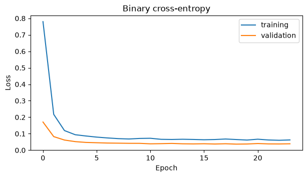
The network outputs the probability of an SEP event. Class weights make each event count about 79 times as much as a non-event in the loss, so the rare class is not ignored. Early stopping restores the epoch with the lowest validation loss.
os.environ["KERAS_BACKEND"] = "torch"
os.environ.setdefault("CUBLAS_WORKSPACE_CONFIG", ":4096:8")  # Deterministic cuBLAS on GPUs.
import keras
import torch
from keras import layers

EPOCHS = 40  # Reduce to 5 or 10 for a quicker run.
keras.utils.set_random_seed(SEED)
torch.use_deterministic_algorithms(True, warn_only=True)
assert keras.backend.backend() == "torch"
# Define the neural network used for SEP occurrence classification.
model = keras.Sequential(
    [
        keras.Input(shape=(x_train.shape[1],)),
        layers.Dense(40, use_bias=False),
        layers.BatchNormalization(),
        layers.ReLU(),
        layers.Dense(30, activation="relu"),
        layers.Dense(1, activation="sigmoid"),
    ]
)
model.compile(optimizer=keras.optimizers.Adam(), loss="binary_crossentropy")
history = model.fit(
    x_train,
    y_train,
    validation_data=(x_validation, y_validation),
    epochs=EPOCHS,
    batch_size=256,
    class_weight={0: 1.0, 1: positive_weight},
    callbacks=[
        keras.callbacks.EarlyStopping(
            monitor="val_loss", patience=5, restore_best_weights=True
        )
    ],
    verbose=0,
)
validation_probabilities = model.predict(x_validation, verbose=0).reshape(-1)
probabilities = model.predict(x_test, verbose=0).reshape(-1)

fig, ax = plt.subplots(figsize=(7, 3.5))
ax.plot(history.history["loss"], label="training")
ax.plot(history.history["val_loss"], label="validation")
ax.set(title="Binary cross-entropy", xlabel="Epoch", ylabel="Loss")
ax.legend()
plt.show()
Evaluate on the supplied test set#
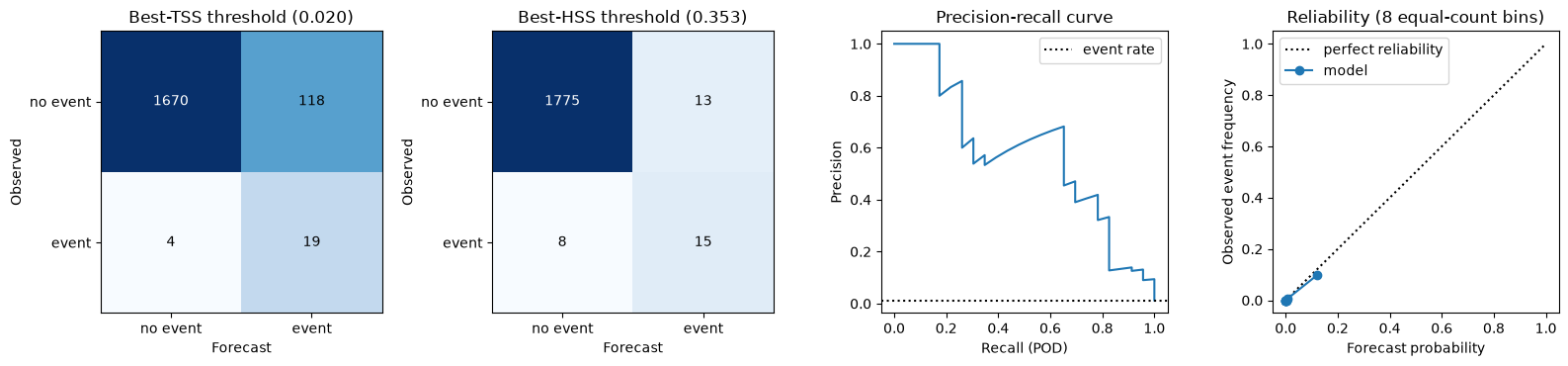
The table compares the model at three thresholds with a forecast of “no event”. The reliability diagram checks whether a forecast probability of \(p\) corresponds to an event frequency of \(p\). Class weighting inflates predicted probabilities, so points below the diagonal are expected.
thresholds = {
    "TSS": choose_threshold(y_validation, validation_probabilities, "TSS"),
    "HSS": choose_threshold(y_validation, validation_probabilities, "HSS"),
}
rows = {
    "always 'no event'": verification_scores(y_test, np.zeros(len(y_test)), 0.5),
    "threshold 0.5": verification_scores(y_test, probabilities, 0.5),
}
for score, value in thresholds.items():
    rows[f"threshold {value:.3f} (best {score} on validation)"] = verification_scores(
        y_test, probabilities, value
    )
table = pd.DataFrame(rows).T
table["PR-AUC"] = [y_test.mean()] + [average_precision_score(y_test, probabilities)] * 3
display(table.round(3))
print("95% bootstrap intervals on the test set:")
display(
    pd.concat(
        {
            f"best-{score} threshold": bootstrap_intervals(y_test, probabilities, value)
            for score, value in thresholds.items()
        },
        axis=1,
    ).round(3)
)

fig, axes = plt.subplots(1, 4, figsize=(16, 3.8))
for axis, (score, value) in zip(axes[:2], thresholds.items()):
    matrix = confusion_matrix(y_test, probabilities >= value, labels=[0, 1])
    axis.imshow(matrix, cmap="Blues", norm="log")
    for (row, column), count in np.ndenumerate(matrix):
        axis.text(
            column, row, str(count), ha="center", va="center",
            color="white" if count > matrix.max() / 10 else "black",
        )
    axis.set(
        title=f"Best-{score} threshold ({value:.3f})",
        xticks=[0, 1], yticks=[0, 1], xticklabels=["no event", "event"],
        yticklabels=["no event", "event"], xlabel="Forecast", ylabel="Observed",
    )
precision, recall, _ = precision_recall_curve(y_test, probabilities)
axes[2].plot(recall, precision)
axes[2].axhline(y_test.mean(), linestyle=":", color="black", label="event rate")
axes[2].set(title="Precision-recall curve", xlabel="Recall (POD)", ylabel="Precision")
axes[2].legend()
observed, forecast = calibration_curve(y_test, probabilities, n_bins=8, strategy="quantile")
axes[3].plot([0, 1], [0, 1], linestyle=":", color="black", label="perfect reliability")
axes[3].plot(forecast, observed, marker="o", label="model")
axes[3].set(
    title="Reliability (8 equal-count bins)",
    xlabel="Forecast probability", ylabel="Observed event frequency",
)
axes[3].legend()
plt.tight_layout()
plt.show()
| hits | misses | false alarms | POD | FAR | TSS | HSS | PR-AUC | |
|---|---|---|---|---|---|---|---|---|
| always 'no event' | 0.0 | 23.0 | 0.0 | 0.000 | 0.000 | 0.000 | 0.000 | 0.013 |
| threshold 0.5 | 10.0 | 13.0 | 7.0 | 0.435 | 0.412 | 0.431 | 0.495 | 0.583 |
| threshold 0.020 (best TSS on validation) | 19.0 | 4.0 | 118.0 | 0.826 | 0.861 | 0.760 | 0.221 | 0.583 |
| threshold 0.353 (best HSS on validation) | 15.0 | 8.0 | 13.0 | 0.652 | 0.464 | 0.645 | 0.582 | 0.583 |
95% bootstrap intervals on the test set:
| best-TSS threshold | best-HSS threshold | |||
|---|---|---|---|---|
| 2.5% | 97.5% | 2.5% | 97.5% | |
| POD | 0.667 | 0.962 | 0.440 | 0.833 |
| FAR | 0.800 | 0.917 | 0.278 | 0.667 |
| TSS | 0.598 | 0.896 | 0.432 | 0.829 |
| HSS | 0.136 | 0.307 | 0.406 | 0.730 |
| PR-AUC | 0.362 | 0.770 | 0.362 | 0.770 |
What the results show#
The threshold matters as much as the model. When events are rare, even a hundred false alarms barely raise the probability of false detection, so maximizing TSS pushes the threshold down until nearly every event is caught and most alarms are false. HSS penalizes false alarms more and selects a higher threshold. Which to use depends on the relative cost of a missed event and a false alarm, a decision for the forecaster rather than the model.
Read the bootstrap intervals before the point estimates: with 23 events, each missed event moves POD by about 0.04. Because the split is by sample rather than by event, all of these scores are likely optimistic.