
SEP Occurrence Forecasting: SHAP Attributions#
The data come from Aminalragia-Giamini et al. (2021), who predicted solar energetic particle (SEP) events from soft X-ray flare measurements. Each sample has 49 standardized predictors and a binary label. The archive has no column names, event identifiers, or timestamps, so two limits apply throughout: predictors cannot be interpreted physically, and samples from the same event may fall on both sides of the train/test split.
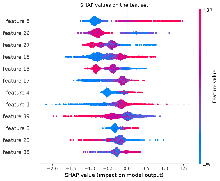
This notebook computes SHAP values for the XGBoost model and checks whether the feature ranking survives a change of random seed.
Imports#
Load the data#
The four pickles are downloaded once and checked against their SHA-256 checksums.
verified dataset: sep-curated
  x_train.pkl (checksum verified)
  x_test.pkl (checksum verified)
  y_train.pkl (checksum verified)
  y_test.pkl (checksum verified)
Split and standardize#
The supplied test set is kept for the final evaluation. A stratified 15% of the supplied training samples becomes the validation set. Trees do not need standardized inputs; we standardize anyway so all SEP notebooks share one preprocessing step.
x_supplied_train = pd.read_pickle(dataset_files["x_train.pkl"]).to_numpy(dtype=np.float32)
x_test_raw = pd.read_pickle(dataset_files["x_test.pkl"]).to_numpy(dtype=np.float32)
y_supplied_train = (
    pd.read_pickle(dataset_files["y_train.pkl"]).to_numpy().reshape(-1).astype(np.int64)
)
y_test = pd.read_pickle(dataset_files["y_test.pkl"]).to_numpy().reshape(-1).astype(np.int64)
feature_names = np.asarray([f"feature {i}" for i in range(x_test_raw.shape[1])])

train_indices, validation_indices = train_test_split(
    np.arange(len(y_supplied_train)),
    test_size=0.15,
    random_state=SEED,
    stratify=y_supplied_train,
)
x_train_raw = x_supplied_train[train_indices]
y_train = y_supplied_train[train_indices]
x_validation_raw = x_supplied_train[validation_indices]
y_validation = y_supplied_train[validation_indices]
# Standardize with statistics from the training part only.
scaler = StandardScaler().fit(x_train_raw)
x_train = scaler.transform(x_train_raw).astype(np.float32)
x_validation = scaler.transform(x_validation_raw).astype(np.float32)
x_test = scaler.transform(x_test_raw).astype(np.float32)

counts = np.bincount(y_train, minlength=2)
positive_weight = counts[0] / counts[1]  # About 79 non-events per event.
print(
    f"train={len(y_train):,} ({counts[1]} events), "
    f"validation={len(y_validation):,} ({y_validation.sum()} events), "
    f"test={len(y_test):,} ({y_test.sum()} events)"
)
print(f"event rate in training: {y_train.mean():.4f}; positive-class weight: {positive_weight:.1f}")
train=13,846 (173 events), validation=2,444 (30 events), test=1,811 (23 events)
event rate in training: 0.0125; positive-class weight: 79.0
Verification scores#
SEP events make up about 1.3% of the samples, so a forecast of “no event” is right 98.7% of the time and useless. We therefore report the scores used in space-weather verification, computed from hits, misses, and false alarms:
POD, the probability of detection: the fraction of events forecast.
FAR, the false-alarm ratio: the fraction of event forecasts that were wrong.
TSS = POD minus the probability of false detection. It ranges from −1 to 1 and does not depend on the event rate.
HSS, the Heidke skill score: accuracy relative to random forecasts with the same event rate.
A probabilistic model needs a threshold to issue yes/no forecasts. We choose two on the validation set, one maximizing TSS and one maximizing HSS, and apply both unchanged to the test set. With only 23 test events, a sample-level bootstrap illustrates sampling variability for this fitted model and threshold; it does not account for dependence between samples from the same event.
def verification_scores(y_true, probability, threshold):
    prediction = probability >= threshold
    tn, fp, fn, tp = confusion_matrix(y_true, prediction, labels=[0, 1]).ravel()
    pod = tp / max(tp + fn, 1)  # Probability of detection (recall).
    pofd = fp / max(fp + tn, 1)  # Probability of false detection.
    far = fp / max(tp + fp, 1)  # False-alarm ratio.
    hss_denominator = (tp + fn) * (fn + tn) + (tp + fp) * (fp + tn)
    return {
        "hits": int(tp), "misses": int(fn), "false alarms": int(fp),
        "POD": pod, "FAR": far, "TSS": pod - pofd,
        "HSS": 2 * (tp * tn - fn * fp) / hss_denominator if hss_denominator else 0.0,
    }


def choose_threshold(y_true, probability, score):
    # Test every distinct decision, including all-positive and all-negative.
    # Ascending thresholds resolve equal scores in favour of the lowest threshold.
    candidates = np.append(np.unique(probability), float(np.max(probability)) + 1.0)
    values = [verification_scores(y_true, probability, t)[score] for t in candidates]
    return float(candidates[int(np.argmax(values))])


def bootstrap_intervals(y_true, probability, threshold, repeats=1000):
    # Resample the test set to show how much the scores move with 23 events.
    rng = np.random.default_rng(SEED)
    draws = []
    for _ in range(repeats):
        sample = rng.integers(0, len(y_true), len(y_true))
        if y_true[sample].sum() == 0:
            continue
        scores = verification_scores(y_true[sample], probability[sample], threshold)
        scores["PR-AUC"] = average_precision_score(y_true[sample], probability[sample])
        draws.append(scores)
    draws = pd.DataFrame(draws)[["POD", "FAR", "TSS", "HSS", "PR-AUC"]]
    return draws.quantile([0.025, 0.975]).T.rename(columns={0.025: "2.5%", 0.975: "97.5%"})
Train a weighted boosted-tree model#
XGBoost fits an ensemble of shallow trees, each correcting the errors of the
ones before it. scale_pos_weight gives events the same weight as in the
neural notebooks, and early stopping on the validation set chooses the
number of trees.
from xgboost import XGBClassifier

ROUNDS = 300  # Reduce to 50 or 100 for a quicker run.
# Define the boosted-tree model used for comparison.
model = XGBClassifier(
    n_estimators=ROUNDS,
    max_depth=6,
    learning_rate=0.05,
    subsample=0.8,
    colsample_bytree=0.8,
    objective="binary:logistic",
    eval_metric="logloss",
    early_stopping_rounds=30,
    scale_pos_weight=positive_weight,
    random_state=SEED,
    n_jobs=2,
)
model.fit(x_train, y_train, eval_set=[(x_validation, y_validation)], verbose=False)
print(f"boosting rounds kept by early stopping: {model.best_iteration + 1} of {ROUNDS}")
validation_probabilities = model.predict_proba(x_validation)[:, 1]
probabilities = model.predict_proba(x_test)[:, 1]
boosting rounds kept by early stopping: 274 of 300
Compute SHAP values#
For each test sample, SHAP splits the model’s output (in log-odds) into one contribution per feature. The beeswarm plot shows the contributions of the twelve most influential features; colour gives the feature value. Because the features are unnamed, this describes what the model relies on, not the physics of SEP production.
import warnings

warnings.filterwarnings("ignore", message="IProgress not found.*")
warnings.filterwarnings("ignore", message="The NumPy global RNG was seeded")
import shap

# Compute model-attribution values for every test sample.
explainer = shap.TreeExplainer(model)
shap_values = np.asarray(explainer.shap_values(x_test))
importance = np.abs(shap_values).mean(axis=0)
shap.summary_plot(
    shap_values, x_test, feature_names=feature_names, max_display=12, show=False
)
plt.title("SHAP values on the test set")
plt.tight_layout()
plt.show()
Is the ranking stable?#
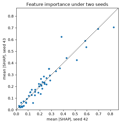
An explanation is only useful if it does not change when nothing important changes. We refit the model with a different random seed, recompute SHAP values, and compare the two importance rankings.
from scipy.stats import spearmanr

refit = XGBClassifier(**{**model.get_params(), "random_state": SEED + 1})
refit.fit(x_train, y_train, eval_set=[(x_validation, y_validation)], verbose=False)
refit_importance = np.abs(np.asarray(shap.TreeExplainer(refit).shap_values(x_test))).mean(axis=0)

top = 10
first_top = set(np.argsort(importance)[-top:])
second_top = set(np.argsort(refit_importance)[-top:])
rank_correlation = spearmanr(importance, refit_importance).statistic
print(f"Spearman rank correlation of mean |SHAP|: {rank_correlation:.3f}")
print(f"features shared by the two top-{top} lists: {len(first_top & second_top)}")

fig, ax = plt.subplots(figsize=(5, 5))
ax.scatter(importance, refit_importance, s=15)
limit = 1.05 * max(importance.max(), refit_importance.max())
ax.plot([0, limit], [0, limit], linestyle=":", color="black")
ax.set(
    xlabel=f"mean |SHAP|, seed {SEED}", ylabel=f"mean |SHAP|, seed {SEED + 1}",
    title="Feature importance under two seeds", xlim=(0, limit), ylim=(0, limit),
)
plt.show()
Spearman rank correlation of mean |SHAP|: 0.959
features shared by the two top-10 lists: 8
What the results show#
The two seed runs share most of their top-ten features, although the full ranking changes. This checks stability across two fits, not physical meaning: what the anonymous features measure cannot be recovered from this archive. Correlated predictors can share or swap attribution.