
Convolutional Network for MNIST: PyTorch#
A dense network treats an image as a list of 784 numbers and ignores which
pixels are neighbours. A convolutional network slides small learned filters
across the image, so the same stroke detector is applied everywhere, and
pooling coarsens the image so that later filters see larger regions. This
notebook trains one on the MNIST digits, with the split used in the
Neural Networks chapter. Set EPOCHS to 1
or 2 in the data cell for a quicker run.
Setup#
The libraries used below.
PyTorch 2.13.0+cu130
Load MNIST and split it#
The 60,000 official training images are split, with a fixed seed and stratified by class, into 50,000 for training and 10,000 for validation. The 10,000 official test images are used once, at the end.
SEED = 42
EPOCHS = 5  # Reduce to 1 or 2 for a quicker run.
BATCH_SIZE = 256
CLASS_NAMES = ['0', '1', '2', '3', '4', '5', '6', '7', '8', '9']

random.seed(SEED)
np.random.seed(SEED)
torch.manual_seed(SEED)
os.environ.setdefault("CUBLAS_WORKSPACE_CONFIG", ":4096:8")  # Deterministic cuBLAS on GPUs.
torch.use_deterministic_algorithms(True, warn_only=True)
DEVICE = torch.device(
    "cuda" if torch.cuda.is_available()
    else "mps" if torch.backends.mps.is_available()
    else "cpu"
)


data_root = Path(
    os.getenv("HELIO_DATA_DIR", Path.home() / ".cache" / "helio-data-methods")
)
development_dataset = datasets.MNIST(data_root, train=True, download=True)
test_dataset = datasets.MNIST(data_root, train=False, download=True)
x_development = development_dataset.data.numpy()
y_development = development_dataset.targets.numpy()
x_test = test_dataset.data.numpy()
y_test = test_dataset.targets.numpy()

all_indices = np.arange(len(y_development))
train_indices, validation_indices = train_test_split(
    all_indices,
    test_size=10000,
    random_state=SEED,
    stratify=y_development,
)
split_signature = hashlib.sha256(
    validation_indices.astype("<i8").tobytes()
).hexdigest()[:16]

# Scale pixel values from 0-255 to 0-1.
x_train = x_development[train_indices].astype("float32") / 255.0
y_train = y_development[train_indices].astype(np.int64)
x_validation = x_development[validation_indices].astype("float32") / 255.0
y_validation = y_development[validation_indices].astype(np.int64)
x_test = x_test.astype("float32") / 255.0
y_test = y_test.astype(np.int64)
x_train = x_train[:, np.newaxis, ...]
x_validation = x_validation[:, np.newaxis, ...]
x_test = x_test[:, np.newaxis, ...]

assert set(train_indices).isdisjoint(validation_indices)
print(
    f"train={len(y_train):,}, validation={len(y_validation):,}, "
    f"test={len(y_test):,}, image shape={x_train.shape[1:]}"
)
train=50,000, validation=10,000, test=10,000, image shape=(1, 28, 28)
Look at the data#
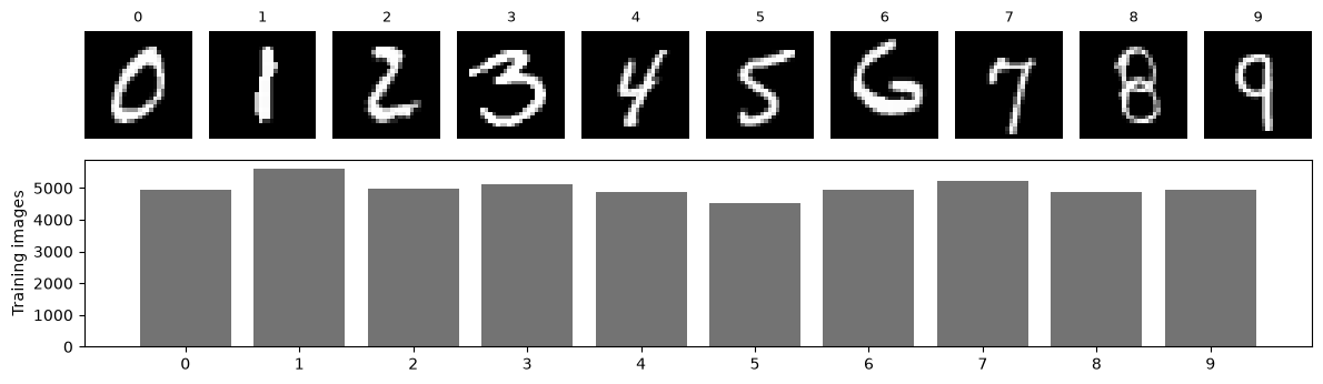
One example per class and the number of training images in each. The classes are balanced, so accuracy is a fair summary of performance.
def as_image(sample):
    # Convert one stored sample to (height, width[, channel]) for plotting.
    if sample.ndim == 1:
        sample = sample.reshape(28, 28)
    if sample.ndim == 3 and sample.shape[0] in (1, 3):
        sample = np.transpose(sample, (1, 2, 0))
    return sample.squeeze()


fig = plt.figure(figsize=(12, 3.6))
grid = fig.add_gridspec(2, 10, height_ratios=[1, 1.2])
for label in range(10):
    axis = fig.add_subplot(grid[0, label])
    image = as_image(x_train[np.flatnonzero(y_train == label)[0]])
    axis.imshow(image, cmap="gray" if image.ndim == 2 else None)
    axis.set_title(CLASS_NAMES[label], fontsize=9)
    axis.axis("off")
counts_axis = fig.add_subplot(grid[1, :])
counts_axis.bar(CLASS_NAMES, np.bincount(y_train, minlength=10), color="0.45")
counts_axis.set(ylabel="Training images")
plt.tight_layout()
plt.show()
Define the model#
Two 3×3 convolution layers with 32 and 64 filters, each followed by a ReLU and 2×2 max pooling, turn a 28×28 image into 64 feature maps of 5×5 pixels. Dropout then zeroes a random quarter of those activations during training, a guard against relying on any single feature. Two dense layers produce ten logits, one unnormalized score per digit.
class ImageClassifier(nn.Module):
    def __init__(self):
        super().__init__()
        self.features = nn.Sequential(
            nn.Conv2d(1, 32, 3), nn.ReLU(), nn.MaxPool2d(2),
            nn.Conv2d(32, 64, 3), nn.ReLU(), nn.MaxPool2d(2), nn.Dropout(0.25),
        )
        self.classifier = nn.Sequential(
            nn.Flatten(), nn.Linear(64 * 5 * 5, 200), nn.ReLU(),
            nn.Linear(200, 150), nn.ReLU(), nn.Dropout(0.5), nn.Linear(150, 10),
        )

    def forward(self, values):
        return self.classifier(self.features(values))


model = ImageClassifier()
print(model)
print(f"trainable parameters: {sum(p.numel() for p in model.parameters()):,}")
ImageClassifier(
  (features): Sequential(
    (0): Conv2d(1, 32, kernel_size=(3, 3), stride=(1, 1))
    (1): ReLU()
    (2): MaxPool2d(kernel_size=2, stride=2, padding=0, dilation=1, ceil_mode=False)
    (3): Conv2d(32, 64, kernel_size=(3, 3), stride=(1, 1))
    (4): ReLU()
    (5): MaxPool2d(kernel_size=2, stride=2, padding=0, dilation=1, ceil_mode=False)
    (6): Dropout(p=0.25, inplace=False)
  )
  (classifier): Sequential(
    (0): Flatten(start_dim=1, end_dim=-1)
    (1): Linear(in_features=1600, out_features=200, bias=True)
    (2): ReLU()
    (3): Linear(in_features=200, out_features=150, bias=True)
    (4): ReLU()
    (5): Dropout(p=0.5, inplace=False)
    (6): Linear(in_features=150, out_features=10, bias=True)
  )
)
trainable parameters: 370,676
Training loop#
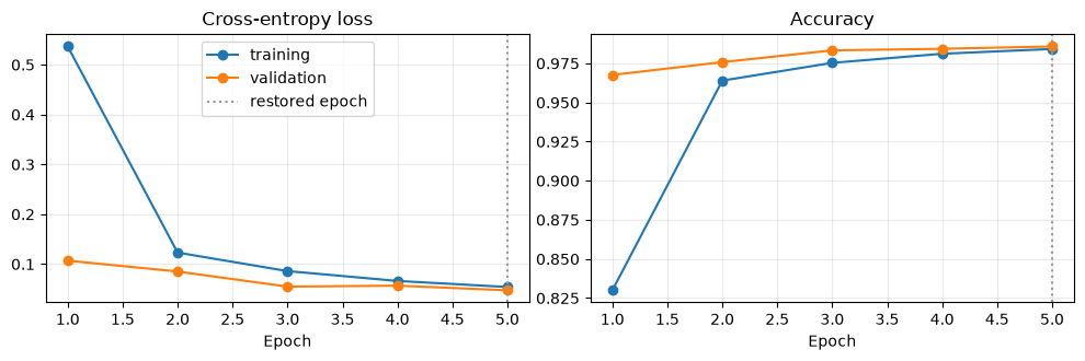
Each epoch passes once over the training images in mini-batches. For each
batch, run_epoch computes the cross-entropy loss (the negative
log-probability given to the correct class), backpropagates its gradient, and
lets the Adam optimizer update the weights. After each epoch fit scores the
validation set, and at the end it restores the weights from the epoch with
the best validation accuracy.
loss_function = nn.CrossEntropyLoss()


def make_loader(images, labels, shuffle=False):
    dataset = TensorDataset(torch.from_numpy(images), torch.from_numpy(labels).long())
    generator = torch.Generator().manual_seed(SEED) if shuffle else None
    return DataLoader(dataset, batch_size=BATCH_SIZE, shuffle=shuffle, generator=generator)


def run_epoch(model, loader, optimizer=None):
    # One pass over `loader`; the weights are updated only if an optimizer is given.
    training = optimizer is not None
    model.train(training)
    total_loss, correct = 0.0, 0
    with torch.set_grad_enabled(training):
        for images, labels in loader:
            images, labels = images.to(DEVICE), labels.to(DEVICE)
            logits = model(images)
            loss = loss_function(logits, labels)
            if training:
                optimizer.zero_grad()
                loss.backward()
                optimizer.step()
            total_loss += loss.item() * len(labels)
            correct += (logits.argmax(dim=1) == labels).sum().item()
    return total_loss / len(loader.dataset), correct / len(loader.dataset)


def fit(model, epochs, learning_rate=1e-3, train=None, validation=None, verbose=True):
    # Train with Adam and restore the epoch with the best validation accuracy.
    train_loader = make_loader(*(train or (x_train, y_train)), shuffle=True)
    validation_loader = make_loader(*(validation or (x_validation, y_validation)))
    model.to(DEVICE)
    optimizer = torch.optim.Adam(model.parameters(), lr=learning_rate)
    history = {"loss": [], "accuracy": [], "val_loss": [], "val_accuracy": []}
    best_state, best_accuracy = None, -1.0
    for epoch in range(epochs):
        scores = (*run_epoch(model, train_loader, optimizer), *run_epoch(model, validation_loader))
        for key, value in zip(history, scores):
            history[key].append(value)
        if verbose:
            print(
                f"epoch {epoch + 1:2d}: loss={scores[0]:.4f}  accuracy={scores[1]:.4f}  "
                f"val_loss={scores[2]:.4f}  val_accuracy={scores[3]:.4f}"
            )
        if scores[3] > best_accuracy:
            best_accuracy = scores[3]
            best_state = {key: value.detach().clone() for key, value in model.state_dict().items()}
    model.load_state_dict(best_state)
    if verbose:
        best_epoch = int(np.argmax(history["val_accuracy"])) + 1
        print(f"restored epoch {best_epoch} (validation accuracy {best_accuracy:.4f})")
    return history


def predict_classes(model, images):
    model.eval()
    with torch.no_grad():
        return np.concatenate(
            [model(batch.to(DEVICE)).argmax(dim=1).cpu().numpy()
             for (batch, _) in make_loader(images, np.zeros(len(images), dtype=np.int64))]
        )


def plot_history(history, title=None):
    epochs = np.arange(1, len(history["loss"]) + 1)
    best = epochs[int(np.argmax(history["val_accuracy"]))]
    fig, axes = plt.subplots(1, 2, figsize=(10, 3.4))
    for axis, key, label in zip(axes, ("loss", "accuracy"), ("Cross-entropy loss", "Accuracy")):
        axis.plot(epochs, history[key], marker="o", label="training")
        axis.plot(epochs, history[f"val_{key}"], marker="o", label="validation")
        axis.axvline(best, color="0.6", linestyle=":", label="restored epoch")
        axis.set(title=label, xlabel="Epoch")
        axis.grid(alpha=0.25)
    axes[0].legend()
    if title:
        fig.suptitle(title)
    plt.tight_layout()
    plt.show()
history = fit(model, EPOCHS)
plot_history(history)
epoch 1: loss=0.5366 accuracy=0.8300 val_loss=0.1069 val_accuracy=0.9676
epoch 2: loss=0.1230 accuracy=0.9640 val_loss=0.0850 val_accuracy=0.9758
epoch 3: loss=0.0859 accuracy=0.9753 val_loss=0.0548 val_accuracy=0.9833
epoch 4: loss=0.0661 accuracy=0.9811 val_loss=0.0567 val_accuracy=0.9843
epoch  5: loss=0.0540  accuracy=0.9842  val_loss=0.0474  val_accuracy=0.9858
restored epoch 5 (validation accuracy 0.9858)
Evaluate on the test set#
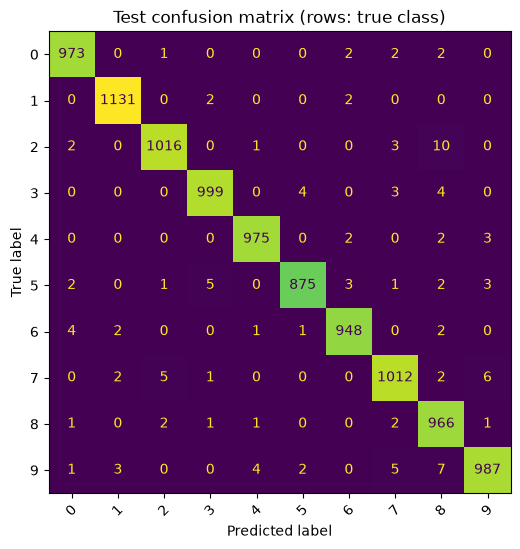
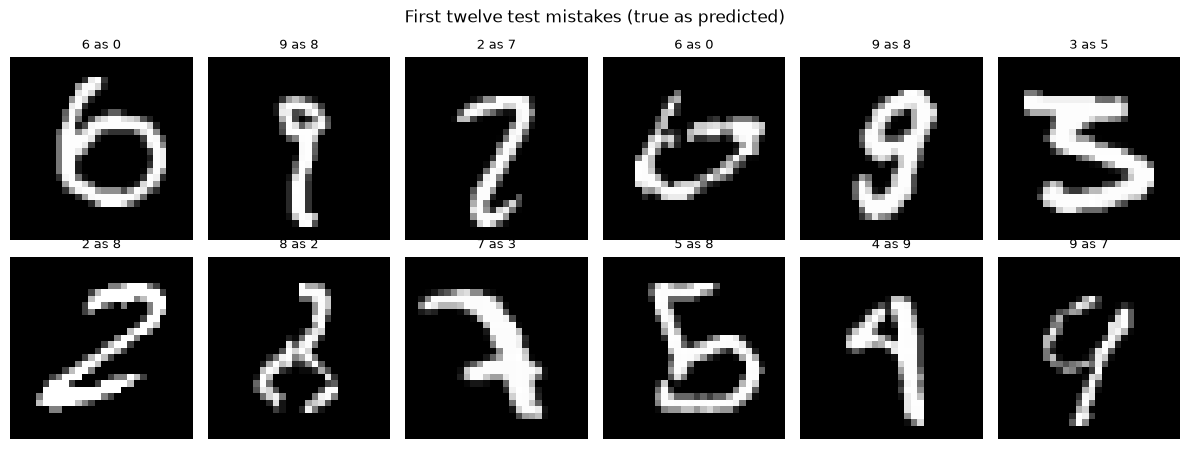
The confusion matrix counts, for each true digit (rows), how often each digit was predicted (columns). The images below are the first twelve test mistakes.
test_predictions = predict_classes(model, x_test)
test_accuracy = accuracy_score(y_test, test_predictions)
cm = confusion_matrix(y_test, test_predictions, labels=np.arange(10))
print(f"test accuracy: {test_accuracy:.4f}")
print(
    classification_report(
        y_test, test_predictions, labels=np.arange(10),
        target_names=CLASS_NAMES, digits=3, zero_division=0,
    )
)

fig, ax = plt.subplots(figsize=(7, 6))
ConfusionMatrixDisplay(cm, display_labels=CLASS_NAMES).plot(
    ax=ax, colorbar=False, values_format="d", xticks_rotation=45
)
ax.set_title("Test confusion matrix (rows: true class)")
plt.show()

mistakes = np.flatnonzero(test_predictions != y_test)[:12]
fig, axes = plt.subplots(2, 6, figsize=(12, 4.6))
for axis in axes.flat:
    axis.axis("off")
for axis, index in zip(axes.flat, mistakes):
    image = as_image(x_test[index])
    axis.imshow(image, cmap="gray" if image.ndim == 2 else None)
    axis.set_title(f"{CLASS_NAMES[y_test[index]]} as {CLASS_NAMES[test_predictions[index]]}", fontsize=9)
fig.suptitle("First twelve test mistakes (true as predicted)")
plt.tight_layout()
plt.show()
test accuracy: 0.9882
              precision    recall  f1-score   support

           0      0.990     0.993     0.991       980
           1      0.994     0.996     0.995      1135
           2      0.991     0.984     0.988      1032
           3      0.991     0.989     0.990      1010
           4      0.993     0.993     0.993       982
           5      0.992     0.981     0.986       892
           6      0.991     0.990     0.990       958
           7      0.984     0.984     0.984      1028
           8      0.969     0.992     0.980       974
           9      0.987     0.978     0.983      1009

    accuracy                          0.988     10000
   macro avg      0.988     0.988     0.988     10000
weighted avg      0.988     0.988     0.988     10000
What the results show#
The convolutional network misclassifies roughly one test digit in a hundred, fewer than half the errors of the dense network in the Neural Networks chapter after the same number of epochs. Weight sharing is the reason: a filter that detects a stroke in one corner detects it everywhere. Many of the remaining mistakes are digits a person would also hesitate over.
Try it yourself#
Change one choice at a time and keep the data split and evaluation unchanged:
change the first convolution from 32 to 64 filters and compare accuracy with parameter count.
compare 3×3 and 5×5 kernels; the dense layer’s input size changes, so print the feature-map shape first.
remove the dropout layers and watch the gap between training and validation loss.