
Dense Neural Network for MNIST: Keras 3#
A neural network is a chain of simple functions with adjustable weights. Training adjusts those weights so the network’s output for each input moves closer to the known answer. This notebook trains a small dense network to recognize handwritten digits from the MNIST collection, and goes through each step: preparing the data, defining the network, the training loop, and an honest evaluation. The Neural Networks chapter gives an overview; the PyTorch version writes the same loop out by hand.
Training runs for five epochs, about a minute on a laptop CPU. Set EPOCHS
to 1 or 2 in the data cell for a quicker run.
Keras and PyTorch#
This notebook runs the Keras 3 API on the PyTorch backend. compile() sets
the optimizer and loss, and fit() runs the loop over batches and epochs
that the PyTorch version writes by hand.
Setup#
The libraries used below.
Keras 3.15.1, backend torch, PyTorch 2.13.0+cu130
Load MNIST and split it#
MNIST contains 70,000 grayscale images of handwritten digits, 28×28 pixels each, divided by its authors into 60,000 training and 10,000 test images. We split the training images again, with a fixed seed and stratified by digit:
50,000 training images, used to fit the weights;
10,000 validation images, used to watch for overfitting while we make choices about the model;
the 10,000 official test images, used once, after all choices are made, to estimate how the model will do on new digits.
SEED = 42
EPOCHS = 5  # Reduce to 1 or 2 for a quicker run.
BATCH_SIZE = 128  # Images per weight update.

keras.utils.set_random_seed(SEED)
torch.use_deterministic_algorithms(True, warn_only=True)

(x_development, y_development), (x_test, y_test) = keras.datasets.mnist.load_data()

all_indices = np.arange(len(y_development))
train_indices, validation_indices = train_test_split(
    all_indices,
    test_size=10_000,
    random_state=SEED,
    stratify=y_development,
)
split_signature = hashlib.sha256(
    validation_indices.astype("<i8").tobytes()
).hexdigest()[:16]

# Scale pixel values from 0-255 to 0-1.
x_train = x_development[train_indices].astype("float32") / 255.0
y_train = y_development[train_indices]
x_validation = x_development[validation_indices].astype("float32") / 255.0
y_validation = y_development[validation_indices]
x_test = x_test.astype("float32") / 255.0

assert set(train_indices).isdisjoint(validation_indices)
print(
    f"train={len(y_train):,}, validation={len(y_validation):,}, "
    f"test={len(y_test):,}, image shape={x_train.shape[1:]}"
)
train=50,000, validation=10,000, test=10,000, image shape=(28, 28)
Look at the data#
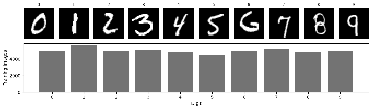
One example of each digit and the number of training images per digit. The classes are nearly balanced, so accuracy is a fair summary of performance.
fig = plt.figure(figsize=(12, 3.6))
grid = fig.add_gridspec(2, 10, height_ratios=[1, 1.2])
for digit in range(10):
    axis = fig.add_subplot(grid[0, digit])
    axis.imshow(x_train[np.flatnonzero(y_train == digit)[0]], cmap="gray")
    axis.set_title(str(digit), fontsize=9)
    axis.axis("off")
counts_axis = fig.add_subplot(grid[1, :])
counts_axis.bar(np.arange(10), np.bincount(y_train, minlength=10), color="0.45")
counts_axis.set(xticks=np.arange(10), xlabel="Digit", ylabel="Training images")
plt.tight_layout()
plt.show()
Define the network#
The network flattens each image into 784 numbers and passes them through two dense layers of 200 and 150 units. Each unit computes a weighted sum of its inputs plus a bias and applies the ReLU function, \(\max(0, x)\); without such nonlinearities a stack of layers would reduce to a single linear map. Dropout sets half of the second layer’s outputs to zero at random during training, which discourages the network from relying on any one unit. The last layer has ten outputs, the logits: unnormalized scores, one per digit, which a softmax turns into probabilities.
The loss is the cross-entropy, the negative log of the probability the network assigns to the correct digit. Adam is the optimizer: a variant of gradient descent that adapts the step size for each weight.
DROPOUT_RATE = 0.5
model = keras.Sequential(
    [
        keras.Input(shape=(28, 28)),
        layers.Flatten(),
        layers.Dense(200, activation="relu"),
        layers.Dense(150, activation="relu"),
        layers.Dropout(DROPOUT_RATE),
        layers.Dense(10),
    ],
    name="dense_mnist",
)
model.compile(
    optimizer=keras.optimizers.Adam(),
    loss=keras.losses.SparseCategoricalCrossentropy(from_logits=True),
    metrics=["accuracy"],
)
model.summary()
Model: "dense_mnist"
┏━━━━━━━━━━━━━━━━━━━━━━━━━━━━━━━━━┳━━━━━━━━━━━━━━━━━━━━━━━━┳━━━━━━━━━━━━━━━┓
┃ Layer (type)                    ┃ Output Shape           ┃       Param # ┃
┡━━━━━━━━━━━━━━━━━━━━━━━━━━━━━━━━━╇━━━━━━━━━━━━━━━━━━━━━━━━╇━━━━━━━━━━━━━━━┩
│ flatten (Flatten)               │ (None, 784)            │             0 │
├─────────────────────────────────┼────────────────────────┼───────────────┤
│ dense (Dense)                   │ (None, 200)            │       157,000 │
├─────────────────────────────────┼────────────────────────┼───────────────┤
│ dense_1 (Dense)                 │ (None, 150)            │        30,150 │
├─────────────────────────────────┼────────────────────────┼───────────────┤
│ dropout (Dropout)               │ (None, 150)            │             0 │
├─────────────────────────────────┼────────────────────────┼───────────────┤
│ dense_2 (Dense)                 │ (None, 10)             │         1,510 │
└─────────────────────────────────┴────────────────────────┴───────────────┘
Total params: 188,660 (736.95 KB)
Trainable params: 188,660 (736.95 KB)
Non-trainable params: 0 (0.00 B)
Train#
An epoch is one pass over the training images, in batches of 128.
For every batch, fit() computes the logits, the loss, and the gradient of
the loss with respect to every weight (backpropagation), and moves each
weight a small step against its gradient. After each epoch it scores the
validation images. The PyTorch version writes these
steps out explicitly.
history = model.fit(
    x_train,
    y_train,
    validation_data=(x_validation, y_validation),
    epochs=EPOCHS,
    batch_size=BATCH_SIZE,
    verbose=2,
)
history = history.history
Epoch 1/5
391/391 - 2s - 6ms/step - accuracy: 0.8799 - loss: 0.4017 - val_accuracy: 0.9540 - val_loss: 0.1620
Epoch 2/5
391/391 - 2s - 5ms/step - accuracy: 0.9532 - loss: 0.1610 - val_accuracy: 0.9666 - val_loss: 0.1173
Epoch 3/5
391/391 - 2s - 6ms/step - accuracy: 0.9666 - loss: 0.1123 - val_accuracy: 0.9697 - val_loss: 0.1011
Epoch 4/5
391/391 - 2s - 5ms/step - accuracy: 0.9749 - loss: 0.0847 - val_accuracy: 0.9734 - val_loss: 0.0924
Epoch 5/5
391/391 - 2s - 5ms/step - accuracy: 0.9791 - loss: 0.0698 - val_accuracy: 0.9727 - val_loss: 0.0927
Learning curves#
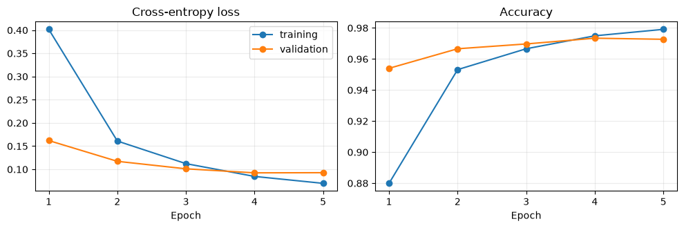
Training loss falls steadily. If validation loss started to rise while training loss kept falling, the network would be memorizing the training images rather than learning digits in general, which is overfitting. In the first epochs validation accuracy is even higher than training accuracy: dropout is off during validation, and the training figure averages over an epoch in which the weights were still improving.
epochs = np.arange(1, len(history["loss"]) + 1)
fig, axes = plt.subplots(1, 2, figsize=(10, 3.4))
for axis, key, label in zip(axes, ("loss", "accuracy"), ("Cross-entropy loss", "Accuracy")):
    axis.plot(epochs, history[key], marker="o", label="training")
    axis.plot(epochs, history[f"val_{key}"], marker="o", label="validation")
    axis.set(title=label, xlabel="Epoch", xticks=epochs)
    axis.grid(alpha=0.25)
axes[0].legend()
plt.tight_layout()
plt.show()
Evaluate on the test set#
The test images are used once, now that the model is fixed.
test_loss, test_accuracy = model.evaluate(x_test, y_test, verbose=0)
test_predictions = model.predict(x_test, batch_size=BATCH_SIZE, verbose=0).argmax(axis=1)
cm = confusion_matrix(y_test, test_predictions, labels=np.arange(10))
print(f"test loss: {test_loss:.4f}")
print(f"test accuracy: {test_accuracy:.4f}")
print(classification_report(y_test, test_predictions, digits=3, zero_division=0))
test loss: 0.0779
test accuracy: 0.9767
              precision    recall  f1-score   support

           0      0.980     0.985     0.982       980
           1      0.991     0.989     0.990      1135
           2      0.982     0.972     0.977      1032
           3      0.976     0.982     0.979      1010
           4      0.976     0.980     0.978       982
           5      0.979     0.983     0.981       892
           6      0.978     0.975     0.976       958
           7      0.988     0.946     0.967      1028
           8      0.976     0.971     0.974       974
           9      0.941     0.984     0.962      1009

    accuracy                          0.977     10000
   macro avg      0.977     0.977     0.977     10000
weighted avg      0.977     0.977     0.977     10000
Which digits are confused?#
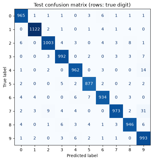
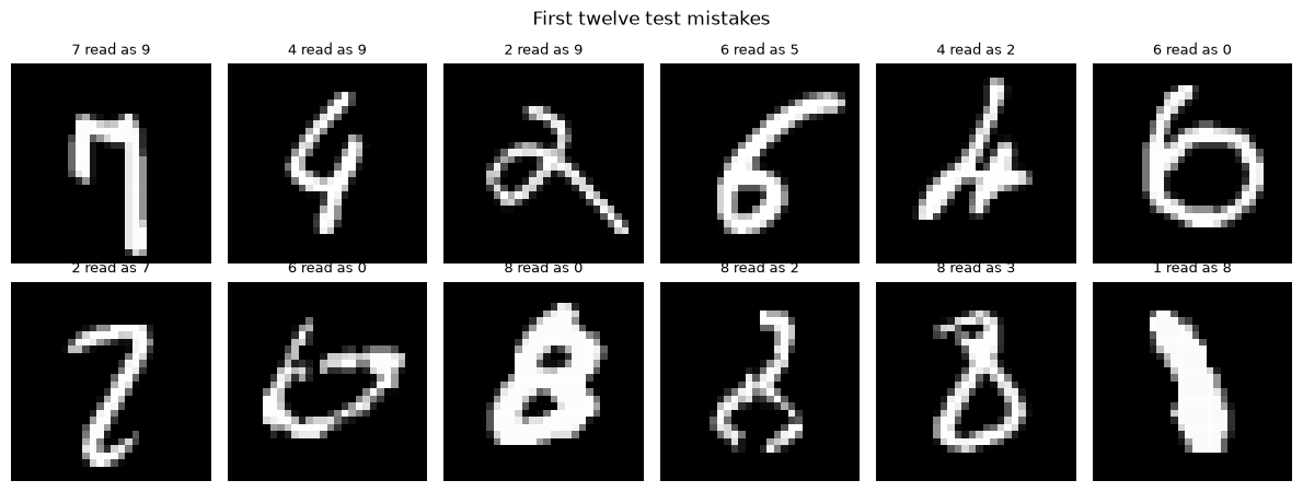
Each row of the confusion matrix is a true digit and each column a predicted one; off-diagonal counts are errors. The images below are the first twelve test mistakes.
fig, ax = plt.subplots(figsize=(6.5, 6))
ConfusionMatrixDisplay(cm, display_labels=np.arange(10)).plot(
    ax=ax, cmap="Blues", colorbar=False
)
ax.set_title("Test confusion matrix (rows: true digit)")
plt.show()

mistakes = np.flatnonzero(test_predictions != y_test)[:12]
fig, axes = plt.subplots(2, 6, figsize=(12, 4.6))
for axis, index in zip(axes.flat, mistakes):
    axis.imshow(x_test[index], cmap="gray")
    axis.set_title(f"{y_test[index]} read as {test_predictions[index]}", fontsize=9)
    axis.axis("off")
fig.suptitle("First twelve test mistakes")
plt.tight_layout()
plt.show()
What the results show#
The network reads about 97.5 of every 100 test digits correctly. Its errors concentrate on a few pairs of similar shapes, and some of the mistakes shown above are hard for a person too. Treating the image as a flat list of pixels discards the fact that neighbouring pixels belong together; the convolutional network uses that structure and makes fewer than half as many errors.
Try it yourself in Keras#
Change one choice at a time and keep the data split and evaluation unchanged:
change dropout from
0.5to0.25and compare the gap between training and validation accuracy.halve the width of both hidden layers and compare the parameter count with the change in accuracy.
set the Adam learning rate to
1e-4and to1e-2and compare the learning curves.