
Hyperparameter Tuning with Optuna: PyTorch#
Hyperparameters are the choices made before training: here the number of
filters in each convolution layer, the width of the dense layer, and the
learning rate. A tuner trains one model per configuration and keeps the
configuration with the best validation accuracy. The test set plays no part
in the search; it scores the selected configuration once at the end. Reduce
TRIALS or SEARCH_EPOCHS for a quicker run.
Setup#
The libraries used below.
PyTorch 2.13.0+cu130
Load MNIST and split it#
The 60,000 official training images are split, with a fixed seed and stratified by class, into 50,000 for training and 10,000 for validation. The 10,000 official test images are used once, at the end.
SEED = 42
BATCH_SIZE = 128
CLASS_NAMES = ['0', '1', '2', '3', '4', '5', '6', '7', '8', '9']

random.seed(SEED)
np.random.seed(SEED)
torch.manual_seed(SEED)
os.environ.setdefault("CUBLAS_WORKSPACE_CONFIG", ":4096:8")  # Deterministic cuBLAS on GPUs.
torch.use_deterministic_algorithms(True, warn_only=True)
DEVICE = torch.device(
    "cuda" if torch.cuda.is_available()
    else "mps" if torch.backends.mps.is_available()
    else "cpu"
)


data_root = Path(
    os.getenv("HELIO_DATA_DIR", Path.home() / ".cache" / "helio-data-methods")
)
development_dataset = datasets.MNIST(data_root, train=True, download=True)
test_dataset = datasets.MNIST(data_root, train=False, download=True)
x_development = development_dataset.data.numpy()
y_development = development_dataset.targets.numpy()
x_test = test_dataset.data.numpy()
y_test = test_dataset.targets.numpy()

all_indices = np.arange(len(y_development))
train_indices, validation_indices = train_test_split(
    all_indices,
    test_size=10000,
    random_state=SEED,
    stratify=y_development,
)
split_signature = hashlib.sha256(
    validation_indices.astype("<i8").tobytes()
).hexdigest()[:16]

# Scale pixel values from 0-255 to 0-1.
x_train = x_development[train_indices].astype("float32") / 255.0
y_train = y_development[train_indices].astype(np.int64)
x_validation = x_development[validation_indices].astype("float32") / 255.0
y_validation = y_development[validation_indices].astype(np.int64)
x_test = x_test.astype("float32") / 255.0
y_test = y_test.astype(np.int64)
x_train = x_train[:, np.newaxis, ...]
x_validation = x_validation[:, np.newaxis, ...]
x_test = x_test[:, np.newaxis, ...]

assert set(train_indices).isdisjoint(validation_indices)
print(
    f"train={len(y_train):,}, validation={len(y_validation):,}, "
    f"test={len(y_test):,}, image shape={x_train.shape[1:]}"
)
train=50,000, validation=10,000, test=10,000, image shape=(1, 28, 28)
Training loop#
Each epoch passes once over the training images in mini-batches. For each
batch, run_epoch computes the cross-entropy loss (the negative
log-probability given to the correct class), backpropagates its gradient, and
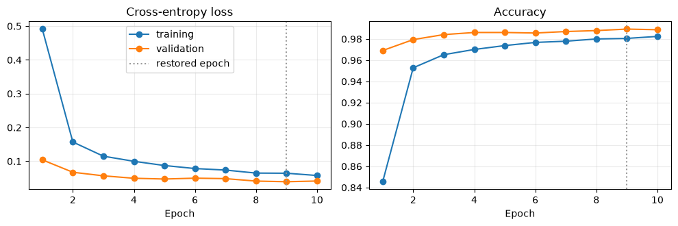
lets the Adam optimizer update the weights. After each epoch fit scores the
validation set, and at the end it restores the weights from the epoch with
the best validation accuracy.
loss_function = nn.CrossEntropyLoss()


def make_loader(images, labels, shuffle=False):
    dataset = TensorDataset(torch.from_numpy(images), torch.from_numpy(labels).long())
    generator = torch.Generator().manual_seed(SEED) if shuffle else None
    return DataLoader(dataset, batch_size=BATCH_SIZE, shuffle=shuffle, generator=generator)


def run_epoch(model, loader, optimizer=None):
    # One pass over `loader`; the weights are updated only if an optimizer is given.
    training = optimizer is not None
    model.train(training)
    total_loss, correct = 0.0, 0
    with torch.set_grad_enabled(training):
        for images, labels in loader:
            images, labels = images.to(DEVICE), labels.to(DEVICE)
            logits = model(images)
            loss = loss_function(logits, labels)
            if training:
                optimizer.zero_grad()
                loss.backward()
                optimizer.step()
            total_loss += loss.item() * len(labels)
            correct += (logits.argmax(dim=1) == labels).sum().item()
    return total_loss / len(loader.dataset), correct / len(loader.dataset)


def fit(model, epochs, learning_rate=1e-3, train=None, validation=None, verbose=True):
    # Train with Adam and restore the epoch with the best validation accuracy.
    train_loader = make_loader(*(train or (x_train, y_train)), shuffle=True)
    validation_loader = make_loader(*(validation or (x_validation, y_validation)))
    model.to(DEVICE)
    optimizer = torch.optim.Adam(model.parameters(), lr=learning_rate)
    history = {"loss": [], "accuracy": [], "val_loss": [], "val_accuracy": []}
    best_state, best_accuracy = None, -1.0
    for epoch in range(epochs):
        scores = (*run_epoch(model, train_loader, optimizer), *run_epoch(model, validation_loader))
        for key, value in zip(history, scores):
            history[key].append(value)
        if verbose:
            print(
                f"epoch {epoch + 1:2d}: loss={scores[0]:.4f}  accuracy={scores[1]:.4f}  "
                f"val_loss={scores[2]:.4f}  val_accuracy={scores[3]:.4f}"
            )
        if scores[3] > best_accuracy:
            best_accuracy = scores[3]
            best_state = {key: value.detach().clone() for key, value in model.state_dict().items()}
    model.load_state_dict(best_state)
    if verbose:
        best_epoch = int(np.argmax(history["val_accuracy"])) + 1
        print(f"restored epoch {best_epoch} (validation accuracy {best_accuracy:.4f})")
    return history


def predict_classes(model, images):
    model.eval()
    with torch.no_grad():
        return np.concatenate(
            [model(batch.to(DEVICE)).argmax(dim=1).cpu().numpy()
             for (batch, _) in make_loader(images, np.zeros(len(images), dtype=np.int64))]
        )


def plot_history(history, title=None):
    epochs = np.arange(1, len(history["loss"]) + 1)
    best = epochs[int(np.argmax(history["val_accuracy"]))]
    fig, axes = plt.subplots(1, 2, figsize=(10, 3.4))
    for axis, key, label in zip(axes, ("loss", "accuracy"), ("Cross-entropy loss", "Accuracy")):
        axis.plot(epochs, history[key], marker="o", label="training")
        axis.plot(epochs, history[f"val_{key}"], marker="o", label="validation")
        axis.axvline(best, color="0.6", linestyle=":", label="restored epoch")
        axis.set(title=label, xlabel="Epoch")
        axis.grid(alpha=0.25)
    axes[0].legend()
    if title:
        fig.suptitle(title)
    plt.tight_layout()
    plt.show()
The search space#
Every combination of the choices below defines one candidate model, 24 in
all. The budget allows TRIALS of them, each trained for up to
SEARCH_EPOCHS epochs and scored by its best validation accuracy.
Optuna’s TPE sampler proposes configurations that resemble the best so far; with only four trials it behaves much like a random search.
TRIALS = 4  # Reduce to 2 for a quicker search.
SEARCH_EPOCHS = 10  # Reduce to 1 or 2 for quicker trials.
SEARCH_SPACE = {
    "filters_1": [16, 32],
    "filters_2": [32, 64],
    "dense_units": [100, 200],
    "learning_rate": [1e-2, 1e-3, 1e-4],
}
Run the search with Optuna#
def build_trial_model(trial):
    filters_1 = trial.suggest_categorical("filters_1", SEARCH_SPACE["filters_1"])
    filters_2 = trial.suggest_categorical("filters_2", SEARCH_SPACE["filters_2"])
    dense_units = trial.suggest_categorical("dense_units", SEARCH_SPACE["dense_units"])
    return nn.Sequential(
        nn.Conv2d(1, filters_1, 3), nn.ReLU(), nn.MaxPool2d(2),
        nn.Conv2d(filters_1, filters_2, 3), nn.ReLU(), nn.MaxPool2d(2),
        nn.Dropout(0.25), nn.Flatten(), nn.Linear(filters_2 * 5 * 5, dense_units),
        nn.ReLU(), nn.Dropout(0.5), nn.Linear(dense_units, 10),
    )


def objective(trial):
    torch.manual_seed(SEED + trial.number)
    model = build_trial_model(trial)
    learning_rate = trial.suggest_categorical("learning_rate", SEARCH_SPACE["learning_rate"])
    history = fit(model, SEARCH_EPOCHS, learning_rate=learning_rate, verbose=False)
    return max(history["val_accuracy"])


study = optuna.create_study(direction="maximize", sampler=optuna.samplers.TPESampler(seed=SEED))
study.optimize(objective, n_trials=TRIALS)
trials = study.trials_dataframe(attrs=("number", "params", "value"))
trials.columns = [column.removeprefix("params_") for column in trials.columns]
display(trials.rename(columns={"value": "best validation accuracy"}).round(4))
| number | dense_units | filters_1 | filters_2 | learning_rate | best validation accuracy | |
|---|---|---|---|---|---|---|
| 0 | 0 | 100 | 32 | 32 | 0.0010 | 0.9893 |
| 1 | 1 | 100 | 16 | 32 | 0.0001 | 0.9693 |
| 2 | 2 | 200 | 16 | 32 | 0.0010 | 0.9888 |
| 3 | 3 | 100 | 32 | 64 | 0.0010 | 0.9892 |
Retrain the selected configuration and evaluate once#
The selected configuration is retrained from scratch with the same epoch
budget, the best validation epoch is restored, and the model is scored on the
test set. optuna.trial.FixedTrial replays the chosen values through the
same model-building function.
torch.manual_seed(SEED)
model = build_trial_model(optuna.trial.FixedTrial(study.best_params))
history = fit(model, SEARCH_EPOCHS, learning_rate=study.best_params["learning_rate"])
plot_history(history)
epoch 1: loss=0.4912 accuracy=0.8455 val_loss=0.1042 val_accuracy=0.9691
epoch 2: loss=0.1570 accuracy=0.9528 val_loss=0.0675 val_accuracy=0.9794
epoch 3: loss=0.1151 accuracy=0.9652 val_loss=0.0570 val_accuracy=0.9841
epoch 4: loss=0.0999 accuracy=0.9701 val_loss=0.0497 val_accuracy=0.9861
epoch 5: loss=0.0875 accuracy=0.9738 val_loss=0.0475 val_accuracy=0.9861
epoch 6: loss=0.0785 accuracy=0.9767 val_loss=0.0500 val_accuracy=0.9856
epoch 7: loss=0.0740 accuracy=0.9779 val_loss=0.0486 val_accuracy=0.9870
epoch 8: loss=0.0651 accuracy=0.9800 val_loss=0.0414 val_accuracy=0.9879
epoch 9: loss=0.0647 accuracy=0.9805 val_loss=0.0395 val_accuracy=0.9893
epoch 10: loss=0.0579  accuracy=0.9824  val_loss=0.0416  val_accuracy=0.9887
restored epoch 9 (validation accuracy 0.9893)
Evaluate on the test set#
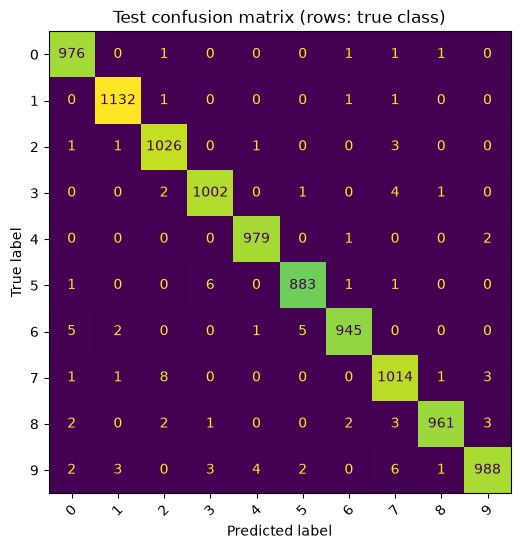
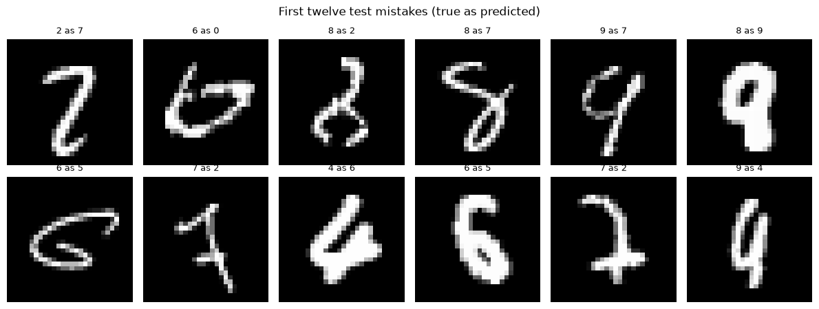
The first twelve test mistakes follow the confusion matrix.
def as_image(sample):
    # Convert one stored sample to (height, width[, channel]) for plotting.
    if sample.ndim == 1:
        sample = sample.reshape(28, 28)
    if sample.ndim == 3 and sample.shape[0] in (1, 3):
        sample = np.transpose(sample, (1, 2, 0))
    return sample.squeeze()


test_predictions = predict_classes(model, x_test)
test_accuracy = accuracy_score(y_test, test_predictions)
cm = confusion_matrix(y_test, test_predictions, labels=np.arange(10))
print(f"test accuracy: {test_accuracy:.4f}")
print(
    classification_report(
        y_test, test_predictions, labels=np.arange(10),
        target_names=CLASS_NAMES, digits=3, zero_division=0,
    )
)

fig, ax = plt.subplots(figsize=(7, 6))
ConfusionMatrixDisplay(cm, display_labels=CLASS_NAMES).plot(
    ax=ax, colorbar=False, values_format="d", xticks_rotation=45
)
ax.set_title("Test confusion matrix (rows: true class)")
plt.show()

mistakes = np.flatnonzero(test_predictions != y_test)[:12]
fig, axes = plt.subplots(2, 6, figsize=(12, 4.6))
for axis in axes.flat:
    axis.axis("off")
for axis, index in zip(axes.flat, mistakes):
    image = as_image(x_test[index])
    axis.imshow(image, cmap="gray" if image.ndim == 2 else None)
    axis.set_title(f"{CLASS_NAMES[y_test[index]]} as {CLASS_NAMES[test_predictions[index]]}", fontsize=9)
fig.suptitle("First twelve test mistakes (true as predicted)")
plt.tight_layout()
plt.show()
test accuracy: 0.9906
              precision    recall  f1-score   support

           0      0.988     0.996     0.992       980
           1      0.994     0.997     0.996      1135
           2      0.987     0.994     0.990      1032
           3      0.990     0.992     0.991      1010
           4      0.994     0.997     0.995       982
           5      0.991     0.990     0.990       892
           6      0.994     0.986     0.990       958
           7      0.982     0.986     0.984      1028
           8      0.996     0.987     0.991       974
           9      0.992     0.979     0.986      1009

    accuracy                          0.991     10000
   macro avg      0.991     0.991     0.991     10000
weighted avg      0.991     0.991     0.991     10000
What the results show#
On MNIST the configurations differ by fractions of a percent once the learning rate is reasonable, so the search mainly rules out the learning rates that are too high or too low. With four trials the ranking of the remaining configurations is not reliable: the differences are comparable to the change caused by a new random seed. A larger budget, or repeated trials per configuration, is needed before a small difference means anything.
Try it yourself#
Change one choice at a time and keep the data split and evaluation unchanged:
rerun the search with a different sampler seed and see whether the same configuration wins.
increase
TRIALSto 12 and check how much the best validation accuracy improves.add dropout rates to the search space.