
Plasma-Sheet Modeling#
This page compares a machine-learning model of Earth’s plasma sheet with the empirical Tsyganenko-Mukai model (TM03). It is adapted from Machine Learning Modeling of Earth’s Plasma Sheet using Multi-Spacecraft Observations (manuscript under review), which uses decades of Geotail and Magnetospheric Multiscale observations to study how data selection, model design, and spacecraft coverage shape statistical models of plasma-sheet density and temperature.
PRIME (Probabilistic Regressor for Input to the Magnetosphere Estimation) is a family of neural networks that predict a quantity together with its uncertainty. The original PRIME propagates solar-wind measurements from L1 to near-Earth space, PRIME-SH models the magnetosheath, and PRIME-PS models plasma-sheet density and ion temperature. Code for all three is in the PRIME repository.
No model is trained here. We load saved PRIME-PS and TM03 outputs and ask two questions:
How do PRIME-PS and the analytical TM03 model compare on the same chronological ion-temperature test samples?
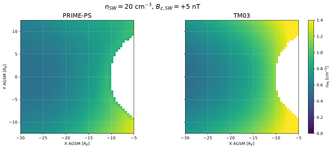
Under one high-density, northward-IMF driving condition, what spatial structure do their equatorial density maps produce?
1. Chronological ion-temperature comparison#
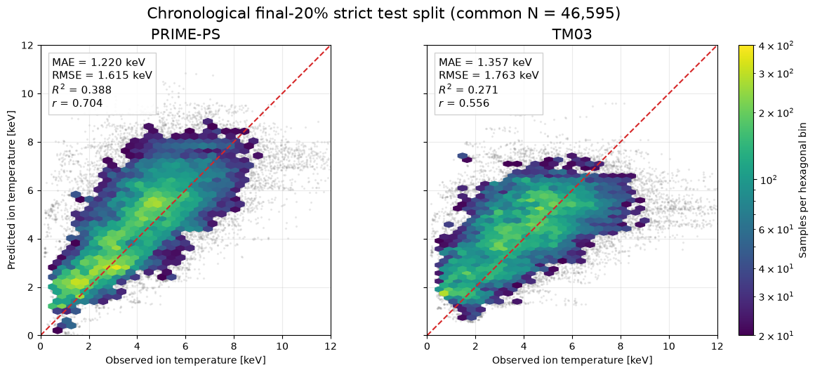
The test set is the final 20% of the observations in time, so it follows the training period. TM03 returns no value for some of these samples; we keep only the 46,595 samples where both models have a prediction, so both are scored on exactly the same population.
observed = results["temperature_observed_kev"]
predictions = {
    "PRIME-PS": results["temperature_prime_ps_kev"],
    "TM03": results["temperature_tm03_kev"],
}
timestamps = results["timestamp_ns"]
if len(observed) != 46_595 or not all(len(values) == len(observed) for values in predictions.values()):
    raise ValueError("Unexpected chronological sample count")


def regression_metrics(y_true, y_pred):
    return {
        "mae_kev": float(mean_absolute_error(y_true, y_pred)),
        "rmse_kev": float(np.sqrt(mean_squared_error(y_true, y_pred))),
        "r2": float(r2_score(y_true, y_pred)),
        "pearson_r": float(np.corrcoef(y_true, y_pred)[0, 1]),
    }


# Evaluate both models on the same chronological sample population.
metrics = {
    model: regression_metrics(observed, predicted)
    for model, predicted in predictions.items()
}
print(f"common chronological samples: {len(observed):,}")
print(f"observations above the displayed 12 keV limit: {(observed > 12).sum():,}")
for model, values in metrics.items():
    print(
        f"{model:8s} | MAE {values['mae_kev']:.3f} keV | "
        f"RMSE {values['rmse_kev']:.3f} keV | R2 {values['r2']:.3f} | "
        f"r {values['pearson_r']:.3f}"
    )
common chronological samples: 46,595
observations above the displayed 12 keV limit: 102
PRIME-PS | MAE 1.220 keV | RMSE 1.615 keV | R2 0.388 | r 0.704
TM03     | MAE 1.357 keV | RMSE 1.763 keV | R2 0.271 | r 0.556
Compare the temperature predictions#
Both panels use the same axes and count scale, so spread, systematic offsets, and behaviour at high temperature can be compared directly. The dashed line marks perfect agreement.
figure, axes = plt.subplots(
    1, 2, figsize=(12.2, 5.2), sharex=True, sharey=True,
    constrained_layout=True,
)
count_norm = LogNorm(vmin=20, vmax=400)  # Share one logarithmic count scale.
hexbin = None

for axis, (model, predicted) in zip(axes, predictions.items()):
    axis.scatter(
        observed, predicted, s=2, color="0.50", alpha=0.12,
        rasterized=True, zorder=1,
    )
    hexbin = axis.hexbin(
        observed, predicted, gridsize=48, mincnt=20,
        cmap="viridis", norm=count_norm, zorder=2,
    )
    axis.plot([0, 12], [0, 12], "--", color="#d62728", linewidth=1.5)
    values = metrics[model]
    metric_text = (
        f"MAE = {values['mae_kev']:.3f} keV\n"
        f"RMSE = {values['rmse_kev']:.3f} keV\n"
        f"$R^2$ = {values['r2']:.3f}\n"
        f"$r$ = {values['pearson_r']:.3f}"
    )
    axis.text(
        0.04, 0.96, metric_text, transform=axis.transAxes,
        va="top", fontsize=11,
        bbox={"facecolor": "white", "edgecolor": "0.8", "alpha": 0.9},
    )
    axis.set_title(model, fontsize=15)
    axis.set_xlabel("Observed ion temperature [keV]")
    axis.set_xlim(0, 12)
    axis.set_ylim(0, 12)
    axis.set_aspect("equal")
    axis.grid(alpha=0.25)

axes[0].set_ylabel("Predicted ion temperature [keV]")
colorbar = figure.colorbar(hexbin, ax=axes, pad=0.02)
colorbar.set_label("Samples per hexagonal bin")
figure.suptitle(
    f"Chronological final-20% strict test split (common N = {len(observed):,})",
    fontsize=16,
)
plt.show()
What the scatter plots show#
PRIME-PS has lower MAE and RMSE and a higher \(R^2\) and correlation than TM03 on the same samples. Neither model reproduces the hottest plasma: both compress the highest observed temperatures toward the middle of the predicted range, so errors grow with temperature.
2. Density structure under high solar-wind density and northward IMF#
This comparison uses no observations. Both models are evaluated on the same equatorial grid for one fixed solar-wind condition, \(n_{SW}=20\,\mathrm{cm}^{-3}\) and \(B_{z,SW}=+5\,\mathrm{nT}\).
The PRIME-PS field was cropped to the TM03 domain, averaged from a 0.1 \(R_E\) to a 0.5 \(R_E\) grid, and smoothed with a one-cell Gaussian filter. A common validity mask and one shared colour scale make the two panels directly comparable.
# Select one common solar-wind condition for both plasma-sheet models.
# Change this key to explore another stored condition.
DENSITY_CASE_KEY = "high_density_northward"  # 20 cm^-3 and +5 nT.

x_edges = results["x_edges_re"]
y_edges = results["y_edges_re"]
density_case_keys = results["density_case_keys"].astype(str).tolist()
density_case_lookup = {
    key: index for index, key in enumerate(density_case_keys)
}
if DENSITY_CASE_KEY not in density_case_lookup:
    raise KeyError(
        f"Unknown density case {DENSITY_CASE_KEY!r}; "
        f"choose from {density_case_keys}"
    )
density_case_index = density_case_lookup[DENSITY_CASE_KEY]
density_maps = {
    "PRIME-PS": results["density_prime_ps_cases_cm3"][density_case_index],
    "TM03": results["density_tm03_cases_cm3"][density_case_index],
}
n_sw = float(results["density_case_n_sw_cm3"][density_case_index])
bz = float(results["density_case_bz_nt"][density_case_index])
smoothing_sigma = float(results["smoothing_sigma_cells"])

if DENSITY_CASE_KEY == "high_density_northward" and (n_sw, bz) != (20.0, 5.0):
    raise ValueError("Unexpected synthetic driving condition")
if not all(grid.shape == (50, 50) for grid in density_maps.values()):
    raise ValueError("Unexpected density-grid shape")
print(f"selected density case: {DENSITY_CASE_KEY}")
print(f"available density cases: {', '.join(density_case_keys)}")

figure, axes = plt.subplots(
    1, 2, figsize=(12.2, 5.0), sharex=True, sharey=True,
    constrained_layout=True,
)
density_mesh = None
for axis, (model, grid) in zip(axes, density_maps.items()):
    density_mesh = axis.pcolormesh(  # Use one color scale for a direct comparison.
        x_edges, y_edges, grid, cmap="viridis",
        vmin=0.0, vmax=1.4, shading="flat",
    )
    axis.set_title(model, fontsize=15)
    axis.set_xlabel(r"X AGSM [$R_E$]")
    axis.set_aspect("equal")
    axis.grid(color="white", linestyle="--", alpha=0.25)
axes[0].set_ylabel(r"Y AGSM [$R_E$]")

colorbar = figure.colorbar(density_mesh, ax=axes, pad=0.02)
colorbar.set_label(r"$n_{PS}$ [cm$^{-3}$]")
figure.suptitle(
    rf"$n_{{SW}}={n_sw:.0f}$ cm$^{{-3}}$, "
    rf"$B_{{z,SW}}={bz:+.0f}$ nT",
    fontsize=16,
)
plt.show()
selected density case: high_density_northward
available density cases: low_density_southward, low_density_northward, high_density_southward, high_density_northward
What the maps show#
PRIME-PS produces a stronger cross-tail, \(Y\)-dependent density structure under this driving condition, while TM03 remains comparatively symmetric. The enhanced structure is dawn-favoring and is consistent with prior observations of plasma entry during northward IMF.
Try it yourself#
Change the scatter limits from 0-12 to 0-19 keV and inspect how the sparse high-temperature tail changes the visual impression. Then ask which metrics would better expose performance for extremes, for example tail-conditioned MAE/RMSE above a threshold chosen in advance, tail bias, or precision and recall for exceeding that threshold.
Rebuild the compact dataset with
--gaussian-sigma 0after extending the preparation script, then compare raw block averages with the lightly smoothed map.In the density-map cell, change
DENSITY_CASE_KEYfrom"high_density_northward"(\(n_{SW}=20\,\mathrm{cm}^{-3}\), \(B_z=+5\,\mathrm{nT}\)) to"high_density_southward"(\(n_{SW}=20\,\mathrm{cm}^{-3}\), \(B_z=-5\,\mathrm{nT}\)) or"low_density_northward"(\(n_{SW}=3\,\mathrm{cm}^{-3}\), \(B_z=+5\,\mathrm{nT}\)). The fourth stored option is"low_density_southward"(\(n_{SW}=3\,\mathrm{cm}^{-3}\), \(B_z=-5\,\mathrm{nT}\)). Keep the same mask, grid, and color limits so the visual comparison remains controlled.
References#
Raptis, S., O’Brien, C., Sorathia, K., Merkin, V., Ohtani, S., Richard, L., Devanandan, A. P., and Wing, S., Machine Learning Modeling of Earth’s Plasma Sheet using Multi-Spacecraft Observations, manuscript under review.
O’Brien, C., Walsh, B. M., Zou, Y., Tasnim, S., Zhang, H., and Sibeck, D. G. (2023), PRIME: a probabilistic neural network approach to solar wind propagation from L1, Frontiers in Astronomy and Space Sciences, 10, 1250779.
O’Brien, C., Walsh, B. M., Zou, Y., Qudsi, R., Tasnim, S., Zhang, H., and Sibeck, D. G. (2024), PRIME-SH: A Data-Driven Probabilistic Model of Earth’s Magnetosheath, Journal of Geophysical Research: Machine Learning and Computation, 1(3), e2024JH000235.
Tsyganenko, N. A., and Mukai, T. (2003), Tail plasma sheet models derived from Geotail particle data, Journal of Geophysical Research: Space Physics, 108(A3).