
Dst Forecasting: PyTorch#
The Dst index measures the depression of the horizontal geomagnetic field at low latitudes, mainly from the storm-time ring current. This notebook forecasts hourly Dst one hour ahead from the previous three hours of solar wind and Dst, and asks a single question: does a small neural network beat persistence, the forecast that nothing changes?
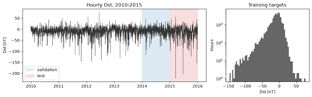
The data are hourly OMNI2 values for 2010-2015. The model trains on
2010-2013, 2014 serves for early stopping, and 2015, which contains the
strongest storm of solar cycle 24, is the test year. See the
Dst Forecasting chapter for an overview. Set EPOCHS to 1 or 2 in
the data cell for a quicker run.
Imports#
A fixed seed makes repeated runs comparable.
Load the OMNI data#
The archived OMNI2 file is downloaded once and checked against its SHA-256 checksum. OMNI solar-wind values are already time-shifted from the upstream spacecraft to the bow-shock nose, so the inputs at hour \(t\) describe the solar wind arriving at Earth at hour \(t\).
data file: omni2_2010-2015.dat (checksum verified)
dataset SHA-256: 18a4ce192bdcc481bdef699a6e11f7f0441b4e933def8dd0c9cd25fc766bcecf
Build forecast windows#
Each sample contains the preceding three hourly values of solar-wind speed \(V\), the GSM \(B_z\) component, field magnitude \(|B|\), and Dst: twelve inputs in all. The target is Dst one hour after the latest input. Windows that span a data gap are dropped, and each year partition is windowed separately so no sample crosses a split boundary. The input scaling is fitted on 2010-2013 only.
HEADERS = [
    "year", "day", "hour", "Bartels", "IMF_spacecraft", "plasma_spacecraft",
    "IMF_av_npoints", "plasma_av_npoints", "av_|B|", "|av_B|",
    "lat_av_B_GSE", "lon_av_B_GSE", "Bx", "By_GSE", "Bz_GSE", "By_GSM",
    "Bz_GSM", "sigma_|B|", "sigma_B", "sigma_Bx", "sigma_By", "sigma_Bz",
    "Tp", "Np", "V_plasma", "phi_V_angle", "theta_V_angle", "Na/Np",
    "P_dyn", "sigma_Tp", "sigma_Np", "sigma_V", "sigma_phi_V",
    "sigma_theta_V", "sigma_Na/Np", "E", "beta", "Ma", "Kp", "R", "Dst",
    "AE", "p_flux_>1MeV", "p_flux_>2MeV", "p_flux_>4MeV",
    "p_flux_>10MeV", "p_flux_>30MeV", "p_flux_>60MeV", "flag", "Ap",
    "f10.7", "PC", "AL", "AU", "M_ms",
]
FILL_VALUES = {
    "av_|B|": 999.9,
    "Bz_GSM": 999.9,
    "V_plasma": 9999.0,
    "Dst": 99999.0,
}
INPUT_COLUMNS = ["V_plasma", "Bz_GSM", "av_|B|", "Dst"]


def read_omni(path):
    frame = pd.read_csv(path, sep=r"\s+", header=None, names=HEADERS)
    frame["timestamp"] = (
        pd.to_datetime(frame["year"].astype(str), format="%Y")
        + pd.to_timedelta(frame["day"] - 1, unit="D")
        + pd.to_timedelta(frame["hour"], unit="h")
    )
    for column, fill_value in FILL_VALUES.items():
        frame.loc[frame[column] == fill_value, column] = np.nan
    return frame


def make_windows(frame, years, history_hours, horizon_hours):
    selected = frame.loc[frame["year"].isin(years)].reset_index(drop=True)
    times = selected["timestamp"].to_numpy(dtype="datetime64[h]")
    values = selected[INPUT_COLUMNS].to_numpy(dtype=np.float32)
    dst = selected["Dst"].to_numpy(dtype=np.float32)
    features, targets, persistence, target_times = [], [], [], []
    for origin in range(history_hours - 1, len(selected) - horizon_hours):
        first = origin - history_hours + 1
        target_index = origin + horizon_hours
        history_times = times[first : origin + 1]
        if not np.all(np.diff(history_times) == np.timedelta64(1, "h")):
            continue
        if times[target_index] - times[origin] != np.timedelta64(horizon_hours, "h"):
            continue
        history = values[first : origin + 1]
        target = dst[target_index]
        if not np.isfinite(history).all() or not np.isfinite(target):
            continue
        features.append(history.reshape(-1))
        targets.append(target)
        persistence.append(history[-1, INPUT_COLUMNS.index("Dst")])
        target_times.append(times[target_index])
    return (
        np.asarray(features, dtype=np.float32),
        np.asarray(targets, dtype=np.float32),
        np.asarray(persistence, dtype=np.float32),
        np.asarray(target_times),
    )


SEED = 42
HISTORY_HOURS = 3
HORIZON_HOURS = 1
EPOCHS = 10  # Reduce to 1 or 2 for a quicker run.
BATCH_SIZE = 128  # Hourly windows per parameter update.

random.seed(SEED)
np.random.seed(SEED)
# Build each year partition independently so information never crosses a split.
frame = read_omni(data_path)
x_train_raw, y_train, persistence_train, time_train = make_windows(
    frame, range(2010, 2014), HISTORY_HOURS, HORIZON_HOURS
)
x_validation_raw, y_validation, persistence_validation, time_validation = make_windows(
    frame, [2014], HISTORY_HOURS, HORIZON_HOURS
)
x_test_raw, y_test, persistence_test, time_test = make_windows(
    frame, [2015], HISTORY_HOURS, HORIZON_HOURS
)

# Estimate the scaling only from 2010–2013.
scaler = StandardScaler().fit(x_train_raw)
x_train = scaler.transform(x_train_raw).astype(np.float32)
x_validation = scaler.transform(x_validation_raw).astype(np.float32)
x_test = scaler.transform(x_test_raw).astype(np.float32)

split_signature = hashlib.sha256(
    time_test.astype("<M8[h]").astype("<i8").tobytes()
    + np.asarray([HISTORY_HOURS, HORIZON_HOURS], dtype="<i8").tobytes()
).hexdigest()[:16]

assert time_train.max() < time_validation.min() < time_test.min()
print(
    f"train={len(y_train):,}, validation={len(y_validation):,}, "
    f"test={len(y_test):,}, history={HISTORY_HOURS} h, horizon={HORIZON_HOURS} h"
)
train=35,043, validation=8,757, test=8,757, history=3 h, horizon=1 h
Look at the data#
Storms are rare: most hours sit within a few tens of nanotesla of zero, so the training targets are dominated by quiet conditions.
fig, axes = plt.subplots(1, 2, figsize=(11, 3.5), gridspec_kw={"width_ratios": [2.2, 1]})
axes[0].plot(frame["timestamp"], frame["Dst"], linewidth=0.5, color="0.2")
axes[0].axvspan(pd.Timestamp("2014-01-01"), pd.Timestamp("2015-01-01"), alpha=0.15, label="validation")
axes[0].axvspan(pd.Timestamp("2015-01-01"), frame["timestamp"].max(), alpha=0.15, color="tab:red", label="test")
axes[0].set(title="Hourly Dst, 2010-2015", ylabel="Dst [nT]")
axes[0].legend(loc="lower left")
axes[1].hist(y_train, bins=60, color="0.4")
axes[1].set(title="Training targets", xlabel="Dst [nT]", yscale="log", ylabel="Hours")
plt.tight_layout()
plt.show()
print(f"hours with Dst < -50 nT: train={np.sum(y_train < -50):,}, test={np.sum(y_test < -50):,}")
hours with Dst < -50 nT: train=915, test=525
Persistence baseline#
For a one-hour forecast, persistence assumes that Dst remains at its value at the forecast origin: \(\widehat{Dst}(t+1) = Dst(t)\). Dst changes slowly outside storms, so this is a demanding reference, and a model is useful only if it beats it.
def regression_metrics(y_true, y_prediction):
    return {
        "MAE [nT]": float(mean_absolute_error(y_true, y_prediction)),
        "RMSE [nT]": float(mean_squared_error(y_true, y_prediction) ** 0.5),
        "R²": float(r2_score(y_true, y_prediction)),
    }


persistence_metrics = regression_metrics(y_test, persistence_test)
print("persistence on 2015:", {key: round(value, 3) for key, value in persistence_metrics.items()})
persistence on 2015: {'MAE [nT]': 3.067, 'RMSE [nT]': 4.766, 'R²': 0.953}
Define the PyTorch model#
Two hidden layers of 50 and 30 ReLU units map the twelve inputs to one Dst value. The loss is the mean squared error.
import torch
from torch import nn
from torch.utils.data import DataLoader, TensorDataset

torch.manual_seed(SEED)
os.environ.setdefault("CUBLAS_WORKSPACE_CONFIG", ":4096:8")  # Deterministic cuBLAS on GPUs.
torch.use_deterministic_algorithms(True, warn_only=True)
DEVICE = torch.device(
    "cuda" if torch.cuda.is_available()
    else "mps" if torch.backends.mps.is_available()
    else "cpu"
)


# Define the neural network used for the Dst forecast.
class DstRegressor(nn.Module):
    def __init__(self, number_inputs):
        super().__init__()
        self.network = nn.Sequential(
            nn.Linear(number_inputs, 50),
            nn.ReLU(),
            nn.Linear(50, 30),
            nn.ReLU(),
            nn.Linear(30, 1),
        )

    def forward(self, values):
        return self.network(values).squeeze(1)


model = DstRegressor(x_train.shape[1]).to(DEVICE)
optimizer = torch.optim.Adam(model.parameters())
loss_function = nn.MSELoss()
print(model)
DstRegressor(
  (network): Sequential(
    (0): Linear(in_features=12, out_features=50, bias=True)
    (1): ReLU()
    (2): Linear(in_features=50, out_features=30, bias=True)
    (3): ReLU()
    (4): Linear(in_features=30, out_features=1, bias=True)
  )
)
Train with early stopping#
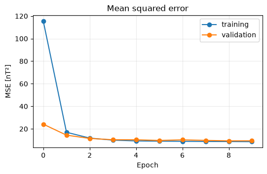
The loop fits on 2010-2013 and checks 2014 after each epoch. Training stops after three epochs without improvement, and the state with the lowest validation loss is restored.
train_loader = DataLoader(
    TensorDataset(torch.from_numpy(x_train), torch.from_numpy(y_train)),
    batch_size=BATCH_SIZE,
    shuffle=True,
    generator=torch.Generator().manual_seed(SEED),
)
x_validation_tensor = torch.from_numpy(x_validation).to(DEVICE)
y_validation_tensor = torch.from_numpy(y_validation).to(DEVICE)
training_loss, validation_loss = [], []
best_state, best_validation, stale_epochs = None, float("inf"), 0

for epoch in range(EPOCHS):
    model.train()
    total = 0.0
    for features, target in train_loader:
        optimizer.zero_grad()
        loss = loss_function(model(features.to(DEVICE)), target.to(DEVICE))
        loss.backward()
        optimizer.step()
        total += loss.item() * len(target)
    training_loss.append(total / len(train_loader.dataset))
    model.eval()
    with torch.no_grad():
        current_validation = loss_function(
            model(x_validation_tensor), y_validation_tensor
        ).item()
    validation_loss.append(current_validation)
    if current_validation < best_validation:
        best_validation, stale_epochs = current_validation, 0
        best_state = {name: value.detach().clone() for name, value in model.state_dict().items()}
    else:
        stale_epochs += 1
        if stale_epochs >= 3:
            break

model.load_state_dict(best_state)
fig, ax = plt.subplots(figsize=(6, 3.5))
ax.plot(training_loss, marker="o", label="training")
ax.plot(validation_loss, marker="o", label="validation")
ax.set(title="Mean squared error", xlabel="Epoch", ylabel="MSE [nT²]")
ax.legend()
ax.grid(alpha=0.25)
plt.show()
Evaluate on 2015#
The test year is used once, after training is complete. Storm hours (Dst < -50 nT) are scored separately, because an overall RMSE is dominated by quiet time.
model.eval()
with torch.no_grad():
    predictions = model(torch.from_numpy(x_test).to(DEVICE)).cpu().numpy()

model_metrics = regression_metrics(y_test, predictions)
# MSE skill score: the fraction of persistence's squared error that the model removes.
persistence_skill = 1.0 - model_metrics["RMSE [nT]"] ** 2 / persistence_metrics["RMSE [nT]"] ** 2
storm_hours = y_test < -50
comparison = pd.DataFrame(
    {
        "neural model": model_metrics,
        "persistence": persistence_metrics,
        "neural model, Dst < -50 nT": regression_metrics(
            y_test[storm_hours], predictions[storm_hours]
        ),
        "persistence, Dst < -50 nT": regression_metrics(
            y_test[storm_hours], persistence_test[storm_hours]
        ),
    }
).T
display(comparison.round(3))
print(f"MSE skill score relative to persistence: {persistence_skill:.3f}")
| MAE [nT] | RMSE [nT] | R² | |
|---|---|---|---|
| neural model | 2.559 | 3.714 | 0.971 |
| persistence | 3.067 | 4.766 | 0.953 |
| neural model, Dst < -50 nT | 5.603 | 7.501 | 0.929 |
| persistence, Dst < -50 nT | 7.000 | 10.069 | 0.872 |
MSE skill score relative to persistence: 0.393
Where the errors are#
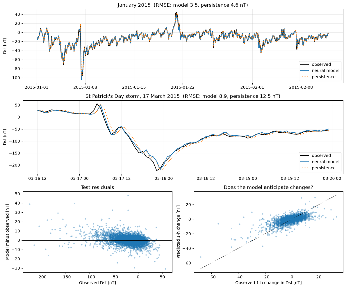
The top panels follow a quiet month and the St Patrick’s Day storm, whose Dst minimum of about -223 nT is the lowest in this six-year record. The lower-left panel shows residuals against observed Dst; the lower-right panel asks whether the model predicts the change in Dst over the next hour, which is the only part of the forecast persistence cannot supply.
def plot_interval(axis, start, stop, title):
    window = (time_test >= np.datetime64(start)) & (time_test < np.datetime64(stop))
    axis.plot(time_test[window], y_test[window], color="black", label="observed")
    axis.plot(time_test[window], predictions[window], label="neural model")
    axis.plot(time_test[window], persistence_test[window], linestyle=":", label="persistence")
    model_rmse = regression_metrics(y_test[window], predictions[window])["RMSE [nT]"]
    persistence_rmse = regression_metrics(y_test[window], persistence_test[window])["RMSE [nT]"]
    axis.set(title=f"{title}  (RMSE: model {model_rmse:.1f}, persistence {persistence_rmse:.1f} nT)", ylabel="Dst [nT]")
    axis.grid(alpha=0.25)
    axis.legend(loc="lower right")


fig = plt.figure(figsize=(12, 10))
grid = fig.add_gridspec(3, 2, height_ratios=[1, 1, 1.1])
plot_interval(fig.add_subplot(grid[0, :]), "2015-01-01", "2015-02-12", "January 2015")
plot_interval(
    fig.add_subplot(grid[1, :]), "2015-03-16T12", "2015-03-20",
    "St Patrick's Day storm, 17 March 2015",
)
residual_axis = fig.add_subplot(grid[2, 0])
residual_axis.scatter(y_test, predictions - y_test, s=6, alpha=0.3)
residual_axis.axhline(0, color="black", linewidth=1)
residual_axis.set(xlabel="Observed Dst [nT]", ylabel="Model minus observed [nT]", title="Test residuals")
change_axis = fig.add_subplot(grid[2, 1])
observed_change = y_test - persistence_test
change_axis.scatter(observed_change, predictions - persistence_test, s=6, alpha=0.3)
limits = [observed_change.min(), observed_change.max()]
change_axis.plot(limits, limits, color="black", linewidth=1, linestyle=":")
change_axis.set(
    xlabel="Observed 1-h change in Dst [nT]", ylabel="Predicted 1-h change [nT]",
    title="Does the model anticipate changes?",
)
plt.tight_layout()
plt.show()

change_correlation = np.corrcoef(observed_change, predictions - persistence_test)[0, 1]
print(f"correlation between observed and predicted 1-h change: {change_correlation:.2f}")
worst = np.argsort(np.abs(y_test - predictions))[-8:][::-1]
display(
    pd.DataFrame(
        {
            "target time": [str(time_test[index])[:13] for index in worst],
            "observed": y_test[worst],
            "neural model": predictions[worst],
            "persistence": persistence_test[worst],
        }
    ).round(1)
)
correlation between observed and predicted 1-h change: 0.63
| target time | observed | neural model | persistence | |
|---|---|---|---|---|
| 0 | 2015-11-03T08 | -21.0 | 27.500000 | 34.0 |
| 1 | 2015-06-23T01 | -131.0 | -91.400002 | -101.0 |
| 2 | 2015-03-17T22 | -223.0 | -183.899994 | -187.0 |
| 3 | 2015-01-07T08 | -21.0 | 11.500000 | 18.0 |
| 4 | 2015-06-22T19 | -53.0 | -20.600000 | -8.0 |
| 5 | 2015-03-17T05 | 56.0 | 25.299999 | 25.0 |
| 6 | 2015-06-22T18 | -8.0 | -37.500000 | -41.0 |
| 7 | 2015-03-17T19 | -165.0 | -135.600006 | -143.0 |
What the results show#
The network beats persistence on 2015 as a whole, with an RMSE of about 3.7 nT against 4.8 nT, and by a wider margin during storm hours. It does so by predicting part of the change over the next hour: the correlation between predicted and observed one-hour changes is about 0.6. The largest errors are the abrupt changes, among them the positive jump at the St Patrick’s Day sudden commencement and the storm minimum itself, which both the network and persistence miss by more than 30 nT. With one hour of lead time and three hours of history, the inputs carry little warning of such changes. One test year with one major storm is a small sample, so the storm-hour scores in particular are uncertain.
Try it yourself#
Change one choice at a time and keep the data split and evaluation unchanged:
change
HORIZON_HOURSfrom 1 to 3 and then 6 while keeping the three-hour input history and 2015 as the final test year; persistence degrades quickly, so watch the skill score.compare three- and six-hour input histories while keeping the one-hour forecast horizon fixed.
replace \(B_z\) with the rectified coupling term \(V B_s\), where \(B_s = -B_z\) for southward field and 0 otherwise, and fit its scaling on training years only.
rebuild the data loading with NASA CDAWeb’s
cdaswsPython API and reproduce the hourly OMNI variables and time range used here.