MNIST with XGBoost

Gradient-boosted trees are the method of choice for many tabular problems. Each tree splits the data on thresholds of individual features; boosting adds trees one at a time, each fitted to the errors of the ensemble so far. Here each 28×28 image is flattened to 784 pixel features, which throws away the spatial layout a convolutional network exploits. The comparison shows what that costs. See Tree Models and Ensembles for the chapter overview.

Setup and data

The MNIST files are downloaded once and verified. The split is the same as in the neural-network notebooks: 50,000 training, 10,000 validation, and 10,000 test images.

Show code cell source

Hide code cell source

import hashlib
import gzip
import importlib.util
import json
import os
import struct
import subprocess
import sys
from pathlib import Path
from urllib.request import urlopen

if importlib.util.find_spec("xgboost") is None:
    subprocess.check_call([sys.executable, "-m", "pip", "install", "-q", "xgboost>=2.1,<4"])

import matplotlib.pyplot as plt
import numpy as np
from sklearn.metrics import (
    ConfusionMatrixDisplay,
    accuracy_score,
    classification_report,
    confusion_matrix,
)
from sklearn.model_selection import train_test_split

SEED = 42
CLASS_NAMES = [str(digit) for digit in range(10)]
raw_root = Path(
    os.getenv("HELIO_DATA_DIR", Path.home() / ".cache" / "helio-data-methods" / "torchvision")
) / "MNIST" / "raw"
raw_root.mkdir(parents=True, exist_ok=True)
mnist_files = {
    "train-images-idx3-ubyte.gz": "440fcabf73cc546fa21475e81ea370265605f56be210a4024d2ca8f203523609",
    "train-labels-idx1-ubyte.gz": "3552534a0a558bbed6aed32b30c495cca23d567ec52cac8be1a0730e8010255c",
    "t10k-images-idx3-ubyte.gz": "8d422c7b0a1c1c79245a5bcf07fe86e33eeafee792b84584aec276f5a2dbc4e6",
    "t10k-labels-idx1-ubyte.gz": "f7ae60f92e00ec6debd23a6088c31dbd2371eca3ffa0defaefb259924204aec6",
}


def fetch_mnist_file(filename, checksum):
    destination = raw_root / filename
    if not destination.exists():
        url = f"https://ossci-datasets.s3.amazonaws.com/mnist/{filename}"
        with urlopen(url, timeout=60) as response:
            destination.write_bytes(response.read())
    actual = hashlib.sha256(destination.read_bytes()).hexdigest()
    if actual != checksum:
        raise RuntimeError(f"MNIST checksum mismatch for {filename}: {actual}")
    return destination


def read_images(path):
    with gzip.open(path, "rb") as stream:
        magic, count, rows, columns = struct.unpack(">IIII", stream.read(16))
        if magic != 2051:
            raise RuntimeError(f"unexpected MNIST image magic number: {magic}")
        return np.frombuffer(stream.read(), dtype=np.uint8).reshape(count, rows, columns)


def read_labels(path):
    with gzip.open(path, "rb") as stream:
        magic, count = struct.unpack(">II", stream.read(8))
        if magic != 2049:
            raise RuntimeError(f"unexpected MNIST label magic number: {magic}")
        return np.frombuffer(stream.read(), dtype=np.uint8, count=count)


resolved_mnist = {
    filename: fetch_mnist_file(filename, checksum)
    for filename, checksum in mnist_files.items()
}
import xgboost as xgb

x_development = read_images(resolved_mnist["train-images-idx3-ubyte.gz"])
y_development = read_labels(resolved_mnist["train-labels-idx1-ubyte.gz"])
x_test = read_images(resolved_mnist["t10k-images-idx3-ubyte.gz"])
y_test = read_labels(resolved_mnist["t10k-labels-idx1-ubyte.gz"])
indices = np.arange(len(y_development))
train_indices, validation_indices = train_test_split(
    indices, test_size=10_000, random_state=SEED, stratify=y_development
)
split_signature = hashlib.sha256(
    validation_indices.astype("<i8").tobytes()
).hexdigest()[:16]
# Flatten each image into 784 pixel features scaled to 0-1.
x_train = x_development[train_indices].reshape(len(train_indices), -1).astype("float32") / 255
y_train = y_development[train_indices]
x_validation = (
    x_development[validation_indices].reshape(len(validation_indices), -1).astype("float32") / 255
)
y_validation = y_development[validation_indices]
x_test = x_test.reshape(len(x_test), -1).astype("float32") / 255
print(f"XGBoost {xgb.__version__}; train={len(y_train):,}, validation={len(y_validation):,}, test={len(y_test):,}")

XGBoost 2.1.4; train=50,000, validation=10,000, test=10,000

Look at the data

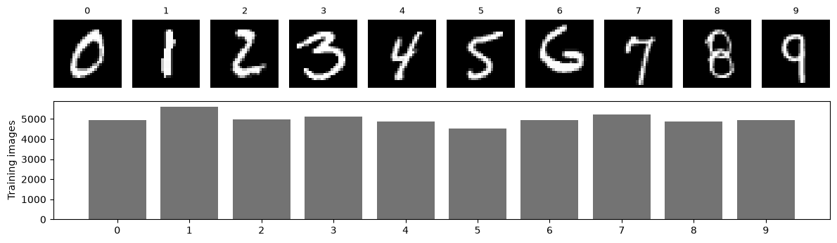
One example per class and the number of training images in each. The classes are balanced, so accuracy is a fair summary of performance.

def as_image(sample):
    # Convert one stored sample to (height, width[, channel]) for plotting.
    if sample.ndim == 1:
        sample = sample.reshape(28, 28)
    if sample.ndim == 3 and sample.shape[0] in (1, 3):
        sample = np.transpose(sample, (1, 2, 0))
    return sample.squeeze()


fig = plt.figure(figsize=(12, 3.6))
grid = fig.add_gridspec(2, 10, height_ratios=[1, 1.2])
for label in range(10):
    axis = fig.add_subplot(grid[0, label])
    image = as_image(x_train[np.flatnonzero(y_train == label)[0]])
    axis.imshow(image, cmap="gray" if image.ndim == 2 else None)
    axis.set_title(CLASS_NAMES[label], fontsize=9)
    axis.axis("off")
counts_axis = fig.add_subplot(grid[1, :])
counts_axis.bar(CLASS_NAMES, np.bincount(y_train, minlength=10), color="0.45")
counts_axis.set(ylabel="Training images")
plt.tight_layout()
plt.show()

Train with early stopping

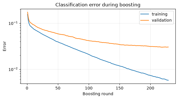
Each boosting round adds one tree per class. eta shrinks each tree’s contribution, max_depth limits how many splits a tree may make, and subsample and colsample_bytree fit each tree on a random 80% of the images and pixels. alpha and lambda penalize large leaf weights. Training stops once the validation error has not improved for 10 rounds.

parameters = {
    "objective": "multi:softprob",
    "num_class": 10,
    "eta": 0.08,
    "max_depth": 6,
    "subsample": 0.8,
    "colsample_bytree": 0.8,
    "alpha": 8,
    "lambda": 2,
    "eval_metric": "merror",
    "seed": SEED,
    "nthread": 2,
}
ROUNDS = 300  # Reduce to 25 or 50 for a quicker run.
dtrain = xgb.DMatrix(x_train, label=y_train)
dvalidation = xgb.DMatrix(x_validation, label=y_validation)
evaluation_log = {}
model = xgb.train(
    parameters,
    dtrain,
    num_boost_round=ROUNDS,
    evals=[(dtrain, "training"), (dvalidation, "validation")],
    early_stopping_rounds=10,
    evals_result=evaluation_log,
    verbose_eval=50,
)
print(f"best round: {model.best_iteration + 1} of {ROUNDS}")

fig, ax = plt.subplots(figsize=(7, 3.4))
for name, log in evaluation_log.items():
    ax.plot(np.arange(1, len(log["merror"]) + 1), log["merror"], label=name)
ax.set(title="Classification error during boosting", xlabel="Boosting round", ylabel="Error", yscale="log")
ax.legend()
ax.grid(alpha=0.25)
plt.show()

[0]	training-merror:0.15484	validation-merror:0.17230

[50]	training-merror:0.03856	validation-merror:0.05820

[100]	training-merror:0.02062	validation-merror:0.04120

[150]	training-merror:0.01160	validation-merror:0.03410

[200]	training-merror:0.00724	validation-merror:0.03100

[227]	training-merror:0.00576	validation-merror:0.03010

best round: 219 of 300

Evaluate on the test set

Predictions use the trees up to the best validation round.

probabilities = model.predict(
    xgb.DMatrix(x_test), iteration_range=(0, model.best_iteration + 1)
)
test_predictions = probabilities.argmax(axis=1)
test_accuracy = accuracy_score(y_test, test_predictions)
cm = confusion_matrix(y_test, test_predictions, labels=np.arange(10))
print(f"test accuracy: {test_accuracy:.4f}")
print(classification_report(y_test, test_predictions, digits=3, zero_division=0))
fig, ax = plt.subplots(figsize=(7, 6))
ConfusionMatrixDisplay(cm).plot(ax=ax, colorbar=False, values_format="d")
ax.set_title("Test confusion matrix (rows: true digit)")
plt.show()

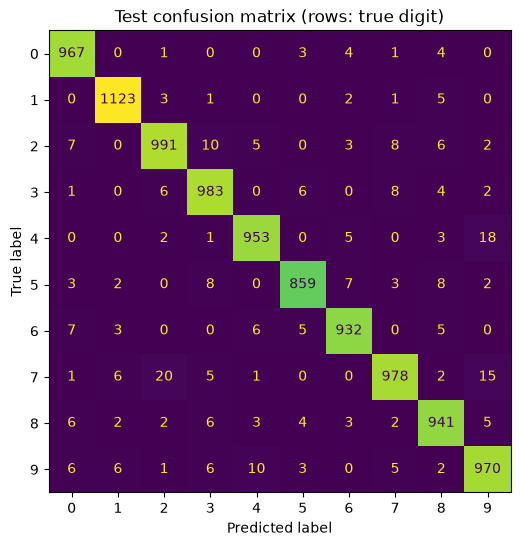
test accuracy: 0.9697
              precision    recall  f1-score   support

           0      0.969     0.987     0.978       980
           1      0.983     0.989     0.986      1135
           2      0.966     0.960     0.963      1032
           3      0.964     0.973     0.968      1010
           4      0.974     0.970     0.972       982
           5      0.976     0.963     0.970       892
           6      0.975     0.973     0.974       958
           7      0.972     0.951     0.962      1028
           8      0.960     0.966     0.963       974
           9      0.957     0.961     0.959      1009

    accuracy                          0.970     10000
   macro avg      0.970     0.969     0.970     10000
weighted avg      0.970     0.970     0.970     10000

What the results show

Boosted trees classify flattened pixels well, but they make two to three times as many errors as the convolutional network on the same split. A tree that splits on pixel 412 learns nothing about pixel 413, so every stroke position has to be learned separately. On tabular data, where features have no spatial arrangement, the comparison usually goes the other way.

Experiment: tree depth

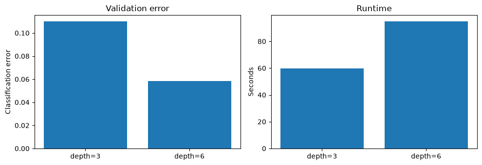
How does maximum tree depth trade validation error against runtime? The two models below use the same training and validation images and the same 50-round ceiling. The test set is not used.

EXAMPLE_ROUNDS = 50  # Reduce to 10 or 25 for a quicker comparison.
EXAMPLE_DEPTHS = [3, 6]
print(f"depths: {EXAMPLE_DEPTHS}; round ceiling: {EXAMPLE_ROUNDS}")

depths: [3, 6]; round ceiling: 50

Show code cell source

Hide code cell source

import time
import pandas as pd


def run_depth_example(depth):
    candidate_parameters = dict(parameters)
    candidate_parameters["max_depth"] = depth
    started = time.perf_counter()
    candidate = xgb.train(
        candidate_parameters,
        dtrain,
        num_boost_round=EXAMPLE_ROUNDS,
        evals=[(dvalidation, "validation")],
        early_stopping_rounds=10,
        verbose_eval=False,
    )
    predictions = candidate.predict(dvalidation).argmax(axis=1)
    return {
        "configuration": f"depth={depth}",
        "validation_error": float(1.0 - accuracy_score(y_validation, predictions)),
        "runtime_seconds": float(time.perf_counter() - started),
        "boosting_rounds": int(candidate.best_iteration + 1),
        "max_depth": depth,
    }

example_results = [run_depth_example(depth) for depth in EXAMPLE_DEPTHS]
example_table = pd.DataFrame(example_results)
display(example_table)
fig, axes = plt.subplots(1, 2, figsize=(10, 3.5))
axes[0].bar(example_table["configuration"], example_table["validation_error"])
axes[0].set(title="Validation error", ylabel="Classification error")
axes[1].bar(example_table["configuration"], example_table["runtime_seconds"])
axes[1].set(title="Runtime", ylabel="Seconds")
plt.tight_layout()
plt.show()

experiment_evidence = {
    "experiment_id": "maximum-tree-depth",
    "configurations": example_table.to_dict(orient="records"),
    "budget": {"rounds": EXAMPLE_ROUNDS, "mode": "compact"},
    "comparison_metrics": ["validation_error", "runtime_seconds", "boosting_rounds"],
    "test_used": False,
}
print("HELIO_EXPERIMENT " + json.dumps(experiment_evidence, sort_keys=True))

	configuration	validation_error	runtime_seconds	boosting_rounds	max_depth
0	depth=3	0.1099	59.671758	50	3
1	depth=6	0.0582	94.795239	50	6

HELIO_EXPERIMENT {"budget": {"mode": "compact", "rounds": 50}, "comparison_metrics": ["validation_error", "runtime_seconds", "boosting_rounds"], "configurations": [{"boosting_rounds": 50, "configuration": "depth=3", "max_depth": 3, "runtime_seconds": 59.67175844099984, "validation_error": 0.1099}, {"boosting_rounds": 50, "configuration": "depth=6", "max_depth": 6, "runtime_seconds": 94.79523877999964, "validation_error": 0.05820000000000003}], "experiment_id": "maximum-tree-depth", "test_used": false}

Try it yourself

• Try depths 2, 4, and 8 and plot validation error against runtime.

• Hold the depth fixed and vary eta between 0.03 and 0.15.

• Change subsample from 0.8 to 0.6 or 1.0 and rerun with a second seed to see how much the error moves.